MODIFICATIONS for the 3 Km Algorithm

While the land and ocean algorithms are fundamentally different from each other, the algorithms that produce the MODIS 3 km product are not scientifically different from those that produce the 10 km product. However, small practical changes had to be made to the land and ocean algorithms to optimize their use for retrieving at a higher spatial resolution. The only differences between the 3 km algorithm and the 10 km algorithm are the way the pixels are organized and the number of pixels required to proceed with a retrieval after all masking and deselection are accomplished.

For the 10 km (nominal at nadir) retrieval, we organize the entire MODIS granule into groups of 20x20 pixels, which we refer to as “retrieval boxes”. The left side of Figure 1 illustrates a 10 km retrieval box outlined in magenta.  The right side of Figure 1 shows a 3 km retrieval box, outlined in red.

Figure 1.  Illustration of the organization of the MODIS pixels into retrieval boxes for  (left) the 10 km product consisting of 20x20 0.5 km pixels within the magenta square and (right) the 3 km product consisting of 6x6 0.5 pixels within the red square.  The small blue squares represent the 0.5 km pixels.  The white rectangles represent pixels identified as cloudy.  The 3 km retrieval box is independent of the 10 km box, and is not a subset.  Here it is shown enlarged.

Figure 2 shows a flow chart showing the separate paths for the 10 km and 3 km retrievals.  The black boxes running along the center of chart identify processes that are identical in both retrievals.  The inputs are identical, as are the masking procedures.  The exact same 0.5 km pixels identified as cloud, sediment etc. in the 10 km algorithm are identified as cloud, sediment etc. in the 3 km algorithm.  The difference is in how the two algorithms make use of these 0.5 km designations.  Once the 3 km algorithm has identified the pixels suitable for retrieval and decided that a sufficient number of these pixels remain, the spectral reflectances are averaged and the inversion continues exactly the same as in the 10 km algorithm.  The same assumptions are used, the same look up tables, the same numerical inversion and the same criteria to determine a good fit.

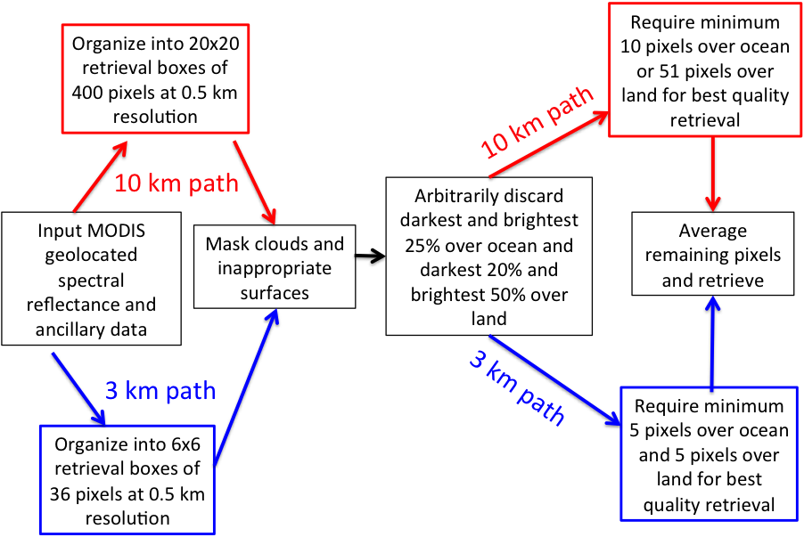
Figure 2.  Flowchart illustrating the different paths of the 10 km (red) and 3 km (blue) retrievals.  The procedures appearing in the black outlined boxes are common to both algorithms.

In the 3 km retrieval the 0.5 km pixels are arranged in retrieval boxes of 6x6 arrays of 36 pixels. Note that in the 3 km retrieval box, the exact same pixels identified as cloudy in the 10 km retrieval box (denoted by the white rectangles) are identified as cloudy in the 3 km box.  This is because both algorithms apply identical criteria to masking undesirable pixels.  The 3 km retrieval applies a similar deselection of pixels at the darkest and brightest ends of the distribution:  25% and 25% over ocean, and 20% and 50% over land. Once these darkest and brightest pixels are discarded, the algorithm averages the remaining pixels to represent conditions in the 3 km retrieval box.  The algorithm requires a minimum of 5 pixels at 0.86 µm over ocean with at least 12 pixels distributed over the other five channels and 5 pixels are required over land in order to continue and make a retrieval.  This is actually a more stringent requirement for ocean (14% of 36), than what is required by the 10 km retrieval (2.5%) for the best quality retrieval.  The requirement over land is about the same in the 3 km retrieval as it is in the 10 km retrieval (14% and 13%, respectively).