6. Provisional evaluation of collection 6 products

Before being run operationally (by MODAPS), the C6 algorithm was tested on 8 months of MODIS-Aqua granules, and compared to the results derived by C5. The testbed consisted of the full months of January and July in 2003, 2008 and 2010, and April and October in 2008. These months were chosen both to highlight aerosol features and to track radiometric stability. Because the radiometric calibration of Terra was still under study during C6 development, the testbed did not include Terra data. This section reports on the comparison between C5 and C6 aerosol products.

 6.1 Comparison of C5 and C6 Global AOD

 

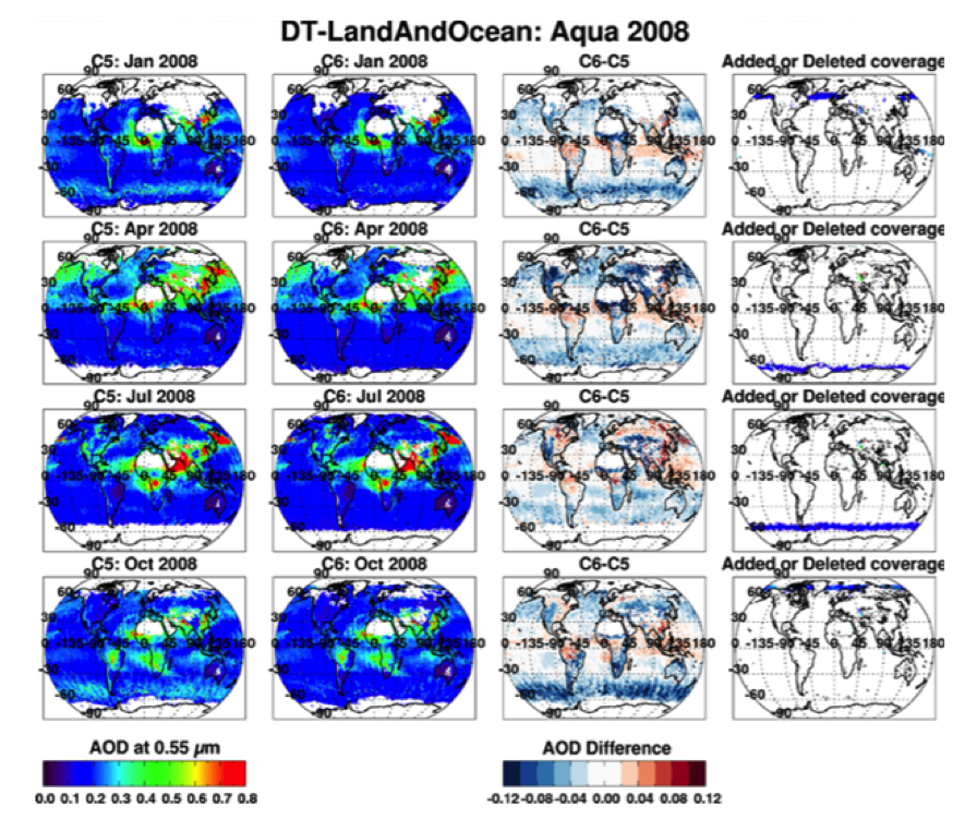
Figure 22: Gridded, monthly averaged 1° x 1° degree AOD (at 0.55 μm) over land and ocean retrieved from Aqua for four months (January, April, July and October) in 2008. For each row (month), the 1st panel is an aggregated product produced from C5, the 2nd panel is from C6 and the 3rd panel is the differences C6–C5. The 4th panel shows the additional AOD coverage (colors) versus deleted coverage (black). From Levy et al, 2013.

Figure 22 shows four months of land and ocean AOD data from January, April, July and October 2008 for both C5 and C6. Over ocean, AOD is generally reduced in C6, due to the inclusion of the multiple wind speed look up table. In the tropics, AOD is increased due to more relaxed cloud screening in the MxD35 cloud masking product. Additionally, more ocean retrievals are possible in C6 because the maximum solar zenith angle allowed to perform AOD retrievals is increased from 72° to 84°. Over land, a changed dependency of the calculation of surface reflectance on NDVI creates the largest change in AOD, causing the AOD over bright surfaces to be decrease and the AOD over dark surfaces to increase. Additionally, global AOD over land is increased due to new calculations of gas corrections, described in Appendix 1.

Figure 23 shows the impact on global AOD from each major change to the algorithm between C5 and C6 for the month of July 2008.  These changes are described more thoroughly Levy et al., 2013. The changes detailed in each panel are:

A. Global high quality AOD for July 2008 using the C5 algorithm.

B. AOD Differences due to using new L1B inputs. These include revised reflectances due to new calibration techniques in the MxD02QKM, MxD02HKM and MxD021KM files, changes in the definition of land and sea due to upgrading to a higher resolution external land/sea mask given in the MxD03 files, and modifications in cloudmasking tests in the MxD35 files.

C. AOD Differences due to updated calculations of central wavelength and Rayleigh optical depth, and from changing the technique of calculating gas absorption from using a moderate resolution spectral database - MODTRAN - to a line-by-line radiative transfer code.

D. AOD differences due to decreasing the quality of cirrus contaminated retrievals. In C5, it was intended that retrievals which may be contaminated by cirrus to have a quality of zero, but there was a bug in the code that allowed the low quality to be overwritten with a higher quality later in the retrieval. In C6, the quality is assigned correctly.

E. AOD differences due to modifications to the land and ocean cloudmasks. The land cloudmask was modified in order to better separate cloud and smoke, resulting in more smoky pixels in C6 being retrieved, and the ocean cloudmask was tightened to counteract the increase in cloud contamination observed in the tropics after using the C6 MxD35 cloudmask.

F. Differences in AOD between C5 and C6.

G. AOD differences due to correcting the VISvs2.11 surface relationship to NDVI_swir over land. Although the theory for how the VISvs2.11 relationship has not changed since C5, in the process of updating the C6 code, it was found that the relationship had not been coded correctly. In C6, the relationship is correct in the code.

I. Changes due to the adapting to the changed land/sea mask provided as upstream input. The C6 land/sea mask is at a 250 m resolution, as opposed to 1 km in C5, which provides more detailed masking of small inland lakes, but also causes much more land to be defined as coastline. To preserve land retrievals over regions with many lakes (e.g., Northern Canada and Finland), the C6 land algorithm now operates on pixels defined as coastline.

J. Differences due to treatment of coastal quality flags. Because retrievals along coastlines are highly susceptible to contamination by unidentified water pixels, retrievals with more then 50% coastline pixels are assigned a QAC of 0.

K. Global high quality AOD for July 2008 using the C6 algorithm.  

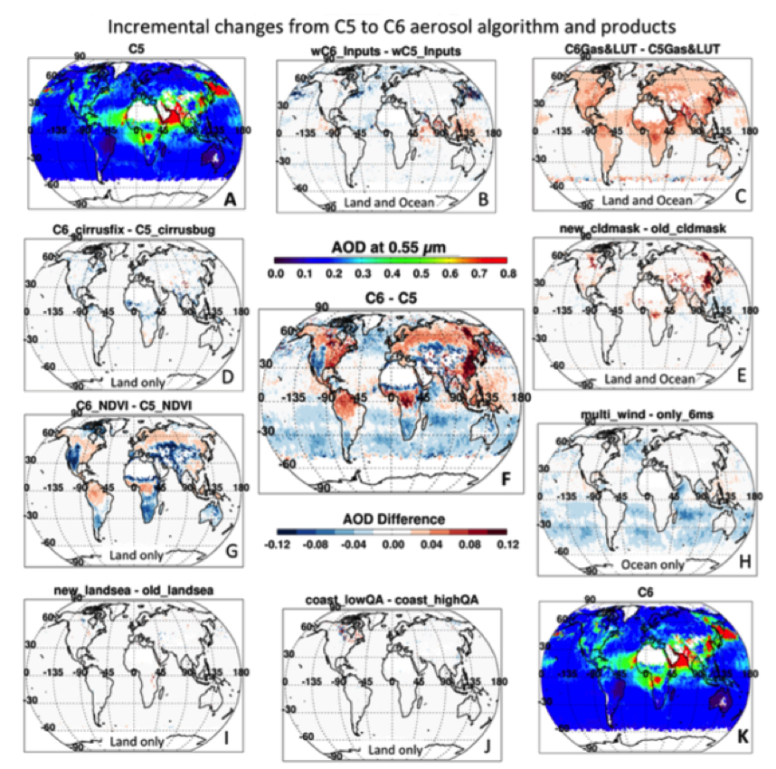
Figure 23: Global, gridded 1° x 1° maps of AOD and AOD differences (new – old) due to major changes to the DT aerosol retrieval algorithm. The example is from July 2008. A) C5 AOD. B) Differences due to using new L1B inputs. C) Differences due to new wavelength and gas absorption coefficients. D) Differences due to correcting a bug in the cirrus cloud masking. E) Differences due to modified cloud masking. G) Differences due to correcting the VISvs2.11 surface relationship to NDVI_swir over land. H) Differences due to including wind speed dependence over ocean. I) Differences due to treatment of land sea masking. J) Differences due to treatment of coastal quality flags. F) Overall differences C6-C5.  K) C6 AOD.  The AOD color scale is for panels A and K, whereas the AOD Difference color scale is for all other panels. From Levy et al., 2013.

6.2 Statistics of C6 vs C5 products

Of most interest to the climate community will be the changes in the statistics of the aerosol products. These include the global mean values and the distribution (histogram) of the values. For the 8 month testbed of MODIS-Aqua granules, the mean 0.55 mm AOD over land increased by 0.02, and the 0.55 µm AOD over ocean decreased by 0.02. However, the change in AOD is dependant on month, with land AOD decreasing in C6 in January and increasing in C6 in July. Table 9 shows the monthly mean AOD statistics over land for the 4 months analyzed in 2008.

6.2.1 Changes to AOD over land :

Table 9 reports global, Level 2 pixel statistics for the four months in 2008, illustrating the following changes:

• –  There are additional granules processed for C6 as compared to C5, which also increases the potential aerosol sampling (15 % increase for Total PixCount).
• –  The net result is approximately 2–3 % additional coverage (Valid PixCount), depending on month.
• –  The QAC (overall Confidence) is reduced. There is near doubling of retrievals with QAC = 0, which better illustrates the confidence related to “coastal” retrievals and cirrus contaminated retrievals. Cases of QAC = 3 (which is the recommended QAC filter over land) are reduced on the order of 10 %.
• –  For the filtered, (QAC = 3) data, global mean AOD decreased sharply in January (from 0.195 to 0.179) and in April (from 0.203 to 0.183), increased during July (from 0.130 to 0.149), and remained nearly constant in October (0.165 to 0.164).

                                                                 Table 9. C5/C6 Comparison of DT

     

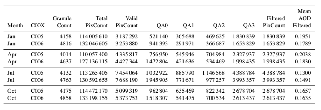
                                                     Land statistics for Aqua; January, April, July and October 2008

 

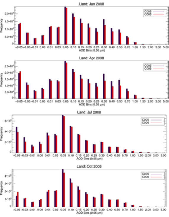
Figure 24: Histograms for global retrieved Level 2 DT-land AOD (at 0.55 mm) from Aqua for four months.  Plotted are data from C5 and C6.

Plotted in Fig. 24 are histograms for the same four months in 2008, showing filtered AOD data for both C5 (blue) and C6 (red). In January and April, we see that, while the number of near-zero AOD retrievals (e.g. less than 0.05) remain constant, the number of moderate (less than 0.4) and high AOD (greater than 0.4) retrievals are reduced. In July, the number of near-zero AOD retrievals is reduced while the higher AOD number is constant. Finally, in October, only the number of moderate AOD cases is impacted (reduced). Because of the negative value bins, a log-normal plot cannot be created, however the selection of bins is suggestive of log scale (adding a constant), and that regardless of season, the median is near 0.05. The large number of negative AOD retrievals will remain a problem for C6. On the other hand, with average global mean AOD being greater than 0.15 in all months, we see that much of the globe is actually very clean (retrieved AOD within ±0.05 of zero).  Returning to Figures 22  and 23, one can see where the C6 algorithm produces the largest absolute changes. In general, changes in AOD are largely positive over the tropics, especially in the northern part of South America and Southeast Asia, while changes are largely negative over mid-latitude continents. Some of these changes are large (0.1). While all factors discussed above in Section 6.1, and illustrated in the different panels of Figure 23, contribute to the net effect seen in Figure 22, the global spatial pattern is very much linked to the changes introduced into C6 from correcting the surface reflectance ratio dependency on NDVI_SWIR (panel g) and to changes in the cloud mask in East Asia and other places with high AOD smoke (panel e). Only in the US Midwest, equatorial Africa and northern Australia, are there changes resulting from the updated assumed aerosol model boundaries.

6.2.2 Changes to AOD and AE over ocean

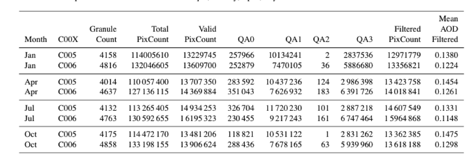
Table 10 reports global, Level 2 pixel AOD statistics for the four months in 2008 over ocean, demonstrating major changes:

• –  The net result is approximately 3–8 % additional coverage (Valid PixCount), depending on month.
• –  The QAC (overall Confidence) is increased. The number of QAC = 0 and QAC = 1 retrievals is decreased, and the number of QAC = 3 retrievals is more than doubled.
• –  For the filtered, QAC ≥ 1 data), global mean AOD decreased in all months (by 0.016–0.019).

                    Table 10. C5/C6 Comparison of DT-ocean statistics for Aqua; January, April, July and October 2008

 

Plotted in Fig. 25 are global histograms of the four months of retrieved AOD data in 2008 for both C5 (blue) and C6 (red), filtered for QAC ≥ 1. We see that, overall, the number of retrievals has increased (7 %) and that there is a significant increase in low AOD cases with a slight decrease in the number of high AOD cases.

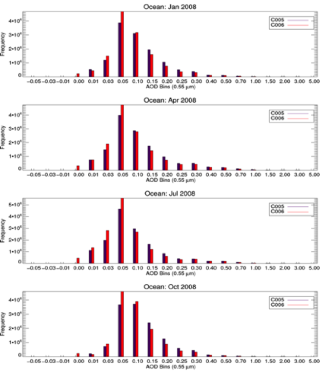
Figure 25: Histograms for global retrieved Level 2 DT-ocean AOD (at 0.55 μm) from Aqua for four months.  Plotted are data from C5 and C6.

In general, changes in AOD are largely negative over the global oceans. As indicated in Table 10, the average decrease for the four months is about 0.018, although there are regions of larger decrease and regions of little decrease (or slight increase). For the most part, the large decreases (∼0.04 or more) are in the mid-latitudes of both summer hemispheres (e.g., the Roaring Forties), where there are systematically higher wind speeds. These decreases in AOD are driven by the addition of variable wind speed in the retrieval (Fig. 23h). The only places where AOD is expected to be higher in C6 than in C5 over ocean are in specific tropical regions that experience an increase in AOD due to modifications to the cloud mask (Fig. 23e) and to the changes in LUT and gas correction.

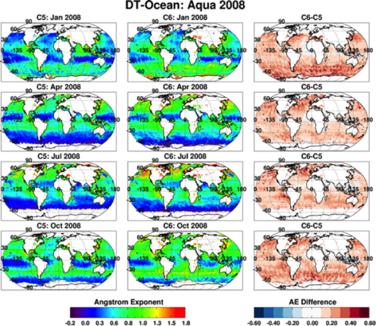
Figure 26: Gridded, monthly averaged 1 × 1 AE (at 0.86/0.55 μm) over ocean retrieved from Aqua for January, April, July and October 2008. Aqua for Jan, Apr, Jul and Oct 2008.. For each row, the left panel is an aggregated product produced from C5, the middle panel is from C6, and the right panel are differences produced from C5, the middle panel is from C6, and the right panel are differences C6-C5.

Focusing now on changes to size parameter over ocean, namely the Angstrom exponent (AE), Fig. 26 plots 1◦ × 1◦ AE, calculated from 0.55 and 0.86 μm for each of the four months of 2008, both collections and the difference between collections. Each monthly mean value is the average of all QAC filtered (QAC≥1) L2 values, within the latitude/longitude grid box, collected during the month. Although this is not necessarily a preferred way of deriving a mean AE value, the plots clearly show how mean AE is expected to increase for C6, especially where AOD is expected to decrease when accounting for wind speed. This indicates that C6 may derive generally smaller-sized aerosol over the global ocean.

6.3 Global mean AOD stability

For C5-derived AOD over ocean, Remer et al. (2008) reported a rather large offset of 0.015 (10%) between the global means of Terra and Aqua, and suggested the discrepancy was due to calibration differences between the two sensors. For the same study, they concluded there was no significant difference between Terra and Aqua over land. However, upon closer examination of the data plots, there is some indication that Terra’s AOD is decreasing, whereas Aqua’s is increasing over time.

Levy et al. (2010) examined the agreement of C5-L MODIS-Aqua and MODIS-Terra AOD against long term (>7 year data record) AERONET sites as a function of time. Figure 27 plots the Error Ratio (ER) for 0.55 μm AOD [(t_MODIS-t_AERO)/EE] calculated for every MODIS/AERONET collocation in our multi-station, seven-year record. There us no trend for Aqua, yet a downward trend for Terra, which is statistically significant. Terra-MODIS seems to be biased high by 0.005 (~5%) early in the mission, flipping to a low bias of similar magnitude sometime after 2004. Although, within the validated EE envelope, this suggests an artificial drift in Terra’s AOD time series.

 

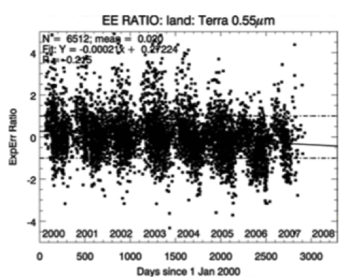
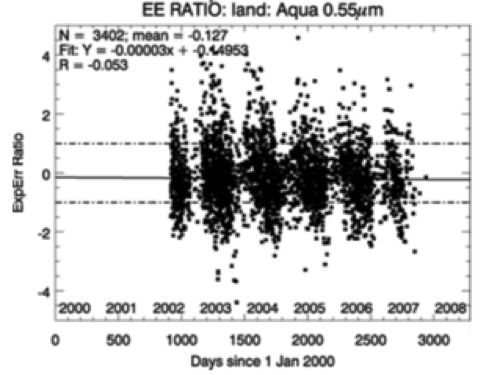
Figure 27: Time series of Error Ratio (ER) of MODIS C005 0.55 μm AOD compared to seven long-term AERONET sites, for Terra (top) and Aqua (bottom). Points between the dashed lines (±1) are cases where MODIS matches AERONET within EE over land (±0.05 ± 0.15%). The solid line is the linear regression. At the top of the plot is text that describes: the number of collocations (N), the regression equation and correlation (R).

In the 4 years between the publication of Levy et al., 2010 and the release of the MODIS Collection 6, significant efforts to understand the suspected calibration drift and modify the calibration procedures for the MODIS instruments were undertaken. Wang et al. (2012) explained how systematic changes in Terra’s blue-band (0.47 μm) calibration could be responsible for the observed NDVI product divergence. Furthermore, our own sensitivity tests demonstrated that a 1–2 % drift in only the blue channel (less than the stated accuracy maintained by MCST) was sufficient to produce a trend in one sensor, or a multi-sensor divergence in the MODIS aerosol products. At the same time, a slight offset in observed red (0.65 μm) and near-IR (0.86 μm) reflectance might be consistent with global offsets over ocean. The ocean color team had previously identified drifting calibration to be a source of error in their data (e.g. Franz et al., 2007; Meister et al., 2012), which could be corrected by vicarious calibration (comparing reported radiances to some ground truth). However, until recently, the problem was thought to be confined to the shortest blue wavelengths (0.41 and 0.44 μm), and was not believed to be a significant problem in the land/aerosol blue channel (0.47 μm) and longer wavelengths. Calibration differences were also suspected to be causing divergences in derived cloud optical properties (e.g. King et al., 2013) between Terra and Aqua.

The trends seen in our dark-target aerosol product, as well as the NDVI and cloud products, clearly indicated that there were also significant issues in longer wavelengths . At that point, the collective MODIS algorithm teams (aerosols, clouds, land surface, ocean, etc.) initiated a bilateral relationship with the MCST. If calibration was going to be updated for C6, then there should be ample opportunity to test and understand why and how changes would be made and how this change would impact the downstream science products including aerosol.

The details of “how” MCST identified and later corrected for the calibration drift, are explained in Sun et al. (2012) and references therein. We focus here on the impacts to the stability of the derived AOD products. We calculate global, monthly mean AOD for each month, for Terra and Aqua separately, and for both C5 and C6 data. The results are plotted as Figure 28, where C5 (C6) is plotted in blue (red), and Terra and Aqua are plotted “T” and “A”. Over land (left panel), it is clear that M_T and M_A do not track each other well for C5, and that M_T>M_A in 2003, but reversed for 2008 and 2010. Even though the retrieval algorithm was updated for C6, for purposes of examining the calibration errors the identical DT-land algorithm is applied to both C5 and C6 data. For C6, we should expect to see better tracking of M_T with M_A, although an offset of ∼0.015 remains. Over the ocean (right panel), there will be a significant drop of 0.018 in all months, however the ∼ 0.01 offset (described by Remer et al., 2008) will remain for C6.

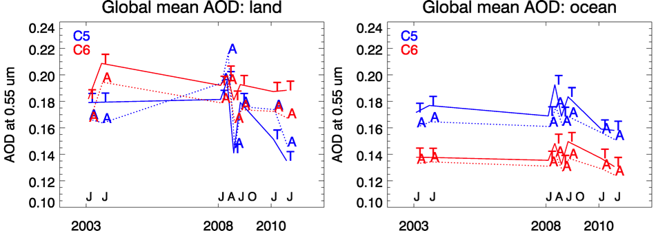
Figure 28: Global monthly mean AOD for DT-land (left) and DT-ocean (right) for eight test months (Jan and July for 2003, 2008 and 2010, plus Apr and Oct 2008) as computed for Terra (T) versus Aqua (A), and C6 (red) versus C5 (blue).

6.4 Comparison of C5 and C6 over-land products with AERONET

Our primary means of provisional validation is comparison with ground-based sunphotometer measurements, specifically, those of AERONET (Holben, et al. 1998).  In ‘sun’ mode, the AERONET instruments measure spectral τ, τ_λ, to within ~0.01 in the MODIS visible and near-IR wavelength regions (Eck et al., 1999) and can be used to derive Fine Weighting (η) by the spectral deconvolution method of O’Neill et al., (2003). The AERONET measured t is easily interpolated to the exact MODIS wavelengths (for example 0.55μm) by quadratic interpolation in log reflectance/log τ space. The AERONET ‘sun-measured’ definition of η differs from either of the MODIS (land or ocean) definitions, but should be correlated with either. The methodology of comparing temporally varying AERONET data with spatially varying MODIS data is described in (Ichoku et al., 2002), and the updated method we apply here is described in Petrenko et. al. (2012).  In the following validation, we use AERONET Level 2.0 data (cloud screened and quality assured for instrument calibration) (Smirnov, et al. 2000). Although North America and Europe provide the most stations in the data base (http://aeronet.gsfc.nasa.gov), all continents (except Antarctica), all oceans and all aerosol types are represented. Remer et al., (2005) provide a comprehensive validation of τ from MODIS C4, whereas Kleidman et al., (2005) provide comparisons of the η product, and Levy et al., (2010) provide a global validation of the C5-L aerosol products.

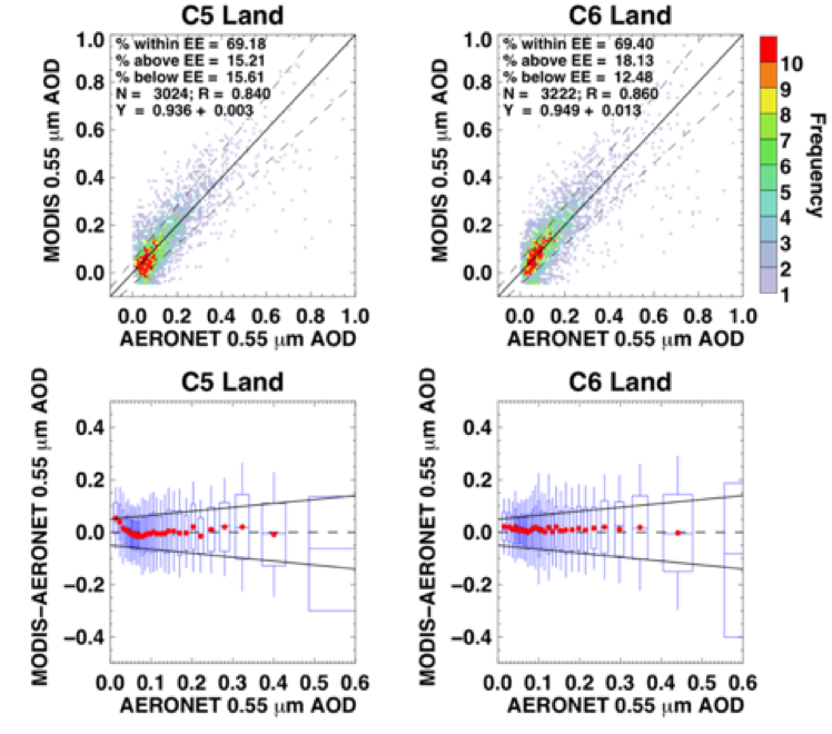
Figure 29: Top row: Frequency scatterplots for AOD at 0.55 μm over dark-land compared to AERONET, plotted from 8 months of Aqua (Jan and July; 2003, 2008 and 2010, and April/September 2008), computed with C5 algorithm (A) and C6 algorithm (B).  One-one lines and EE envelopes ±(0.05 + 15%) are plotted as solid and dashed lines.  Collocation statistics are presented in each panel. Bottom Row: The same information plotted as AOD error (MODIS-AERONET) versus AERONET, broken into equal number bins of AERONET AOD.   One-one line (zero error) is dashed and EE envelopes are solid.   For each box-whisker, its properties and what they represent include: width is 1-σ of the AOD bin, whereas height, whiskers, middle line and red dots are the 1-σ, 2-σ, mean and median of the AOD error, respectively.

In Figure 29, we compare MODIS versus AERONET AOD, for the entire eight months of Aqua test data. Here, we use the revised protocol developed by Petrenko et al. (2012), where satellite and sun photometer are compared within a spatial radius of ±27.5 km and a temporal interval of ±30 min. A valid collocation is one where there are at least 20% of possible MODIS pixels and two sun photometer measurements within the spatial/temporal window. While there is a decrease in total filtered pixel counts between C5 and C6, there is a 6% increase in the number of valid MODIS/AERONET collocations. Although there might be less MODIS sampling in the cloudy tropics (few or no AERONET sites), there is increased MODIS coverage where there are matching AERONET sites (e.g. northern Europe with low sun angles). Although the slope and offset of the regression curve changes slightly between C5 and C6, the high skill at retrieving AERONET-observed AOD is retained. Overall, for C6, the correlation is R = 0.86, and that 69.4 % of MODIS AOD fall within expected uncertainty of ±(0.05 + 15 %). Like Levy et al. (2010), we plot MODIS-AERONET (e.g. MODIS error) compared to equal frequency bins of AERONET AOD. Overall, the pattern is unchanged from C5 to C6, however, there is improvement for the lowest AOD bins. Much of this improvement comes from reversing the NDVI_SWIR dependence, and resulting retrieval of lower AOD over semi-arid regions. Interestingly while there are many retrievals of negative AOD in the histogram (Figure 24), they are constrained to regions (e.g. Australia) where there are few AERONET sites.

6.5 Comparison of ocean products with AERONET

Over ocean, the expected τ error is  smaller than over land. This is because the (non-glint) ocean surface contribution to spectral reflectance can be characterized with a higher level of accuracy than the land surface reflectance. Figure 30 compares QAC filtered (QAC ≥ 1) MODIS τ at 0.55 mm compared to the AERONET τ (quadratic fit to 0.55μm). 

In addition to plotting MODIS versus AERONET, we also display comparisons for MODIS versus the ship-based sun photometers of the Maritime Aerosol Network (MAN; http://aeronet.gsfc.nasa.gov/ new_web/maritime_aerosol_network.html, Smirnov et al., 2009). For each panel, the square symbols (grey and colored) represent frequency of MODIS/AERONET collocations at each ordered pair (0.01 intervals), whereas the black circles are collocations for MODIS versus MAN. Comparison statistics in all panels are for MODIS versus AERONET only. While there was a 6 % increase in total filtered (QAC ≥ 1) pixel counts between C5 and C6, there is a 30 % increase in the number of valid MODIS/AERONET AOD collocations (from 830 to 1141) and a similar increase for MODIS/MAN (33 to 41). There is an improvement in regression slope (from 0.88 to 0.97) and trivial improvement in correlation (from 0.928 to 0.937). Visually, there is slightly less scatter for MAN. The bottom panels of Figure 30 show that the improvement occurs throughout the range of AOD, with high biases at low AOD decreasing and low.  Even after improvements, Fig. 30d clearly shows that there remains a MODIS high bias at low AOD. Also, the scatter for high AOD is significantly larger than the EE of ±(0.03 + 5 %) as determined by previous validation studies (e.g. Remer et al., 2008). Therefore, we take this opportunity to refine the EE envelope for MODIS over ocean to better represent the asymmetry of Figure 30d. Here, we define expected EE for C6 as (+(0.04 + 10 %), −(0.02 + 10 %)), where we also note the asymmetry. These new EE lines are drawn in all panels of Figure 30.

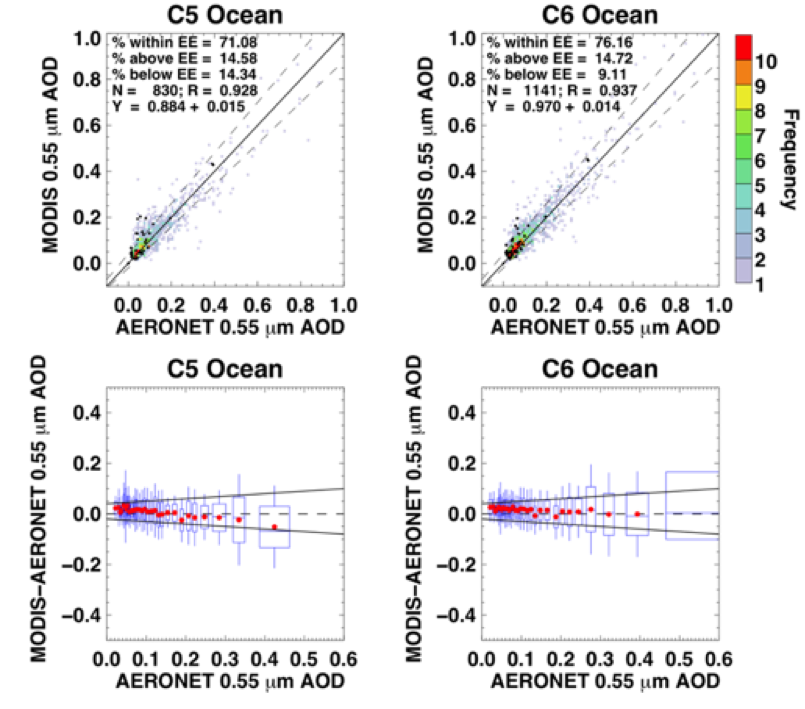
Figure 30: Top row: Frequency scatterplots for AOD at 0.55 μm over DT-ocean compared to AERONET (gray and color dots) and MAN (black dots), plotted from 8 months of Aqua (Jan and July; 2003, 2008 and 2010, and Apr/Sept 2008), computed with C5 algorithm (A) and C6 algorithm (B).  One-one lines and EE envelopes (+(0.04 + 10%), -(0.02 + 10%), asymmetric ) are plotted as solid and dashed lines.  Collocation statistics are presented in each panel. Bottom Row: The same information (AERONET only) plotted as AOD error (MODIS-AERONET) versus AERONET, broken into equal number bins of AERONET AOD.   One-to-one line (zero error) is dashed and EE envelopes are solid.   For each box-whisker, its properties and what they represent include: width is 1-σ of the AOD bin, whereas height, whiskers, middle line and red dots are the 1-σ, 2-σ, mean and median of the AOD error, respectively.

Because definitions of fine-mode fraction (FMF) can be ambiguous (Kleidman et al., 2005), we focus on comparisons of Angstrom Exponent (AE) as recommended by Anderson et al. (2005). Due to the expected accuracy of the sun photometer data, they are interpolated to MODIS wavelengths, rather than vice-versa. Figure 31 shows 22% more collocated points in C6 than in C5. Here, the EE is drawn as ±0.40, which captures nearly 63% of collocations for all values of AE. Resetting at ±0.41 captures 68%. While there is no significant overall improvement for AE comparability in C6, there are fewer cases where MODIS is retrieving the limiting values for AE. This suggests that improved pixel screening or other corrections (Rayleigh, gas) may be providing the DT-ocean retrieval with more consistent information. The same reasoning may be responsible for the decrease in the scatter with relation to MAN-derived AE; that allows the C6 retrieval to make better use of the information.

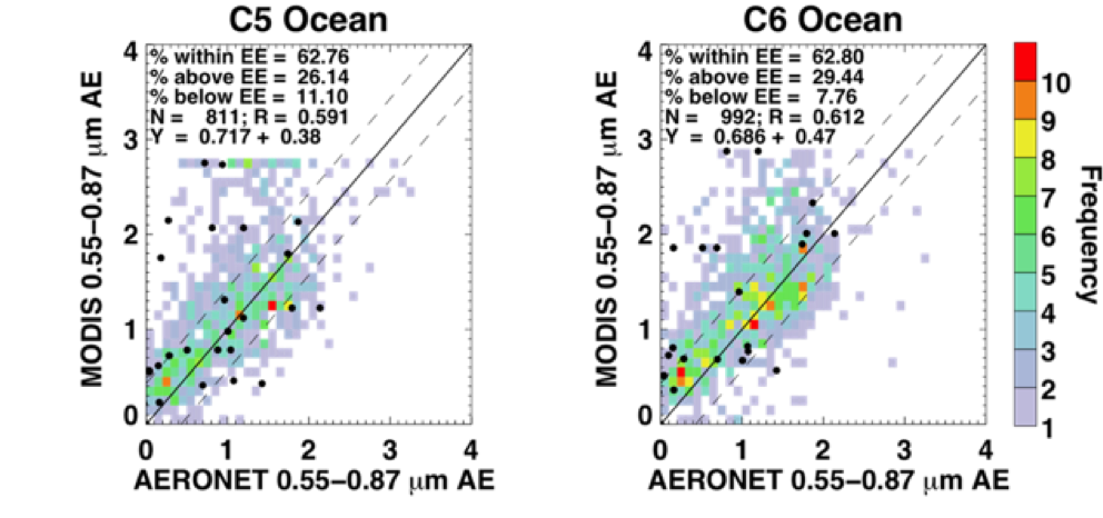
Figure 31: Frequency scatterplots for AE at 0.55/0.86 μm over DT-ocean compared to AERONET (gray and color dots) and MAN (black dots), plotted from 8 months of Aqua (Jan and July; 2003, 2008 and 2010, and Apr/Sept 2008), computed with C5 algorithm (A) and C6 algorithm (B).  One-one lines and EE envelopes (±0.40) are plotted as solid and dashed lines.  Collocation statistics are presented in each panel.