
7. The C6 3 km aerosol product
7.1 Algorithmic adaptations for the 3 km product
While the land and ocean algorithms are fundamentally different from each other, the algorithms that produce the MODIS 3 km product are not logically different from those that produce the 10 km product. However, small practical changes had to be made to the land and ocean algorithms to optimize their use for retrieving at a higher spatial resolution. The only differences between the 3 km algorithm and the 10 km algorithm are the way the pixels are organized and the number of pixels required to proceed with a retrieval after all masking and deselection are accomplished.
For the 10 km (nominal at nadir) retrieval, we organize the entire MODIS granule into groups of 20x20 pixels, which we refer to as “retrieval boxes”. The left side of Figure 32 illustrates a 10 km retrieval box outlined in magenta. The right side of Figure 32 shows a 3 km retrieval box, outlined in red.
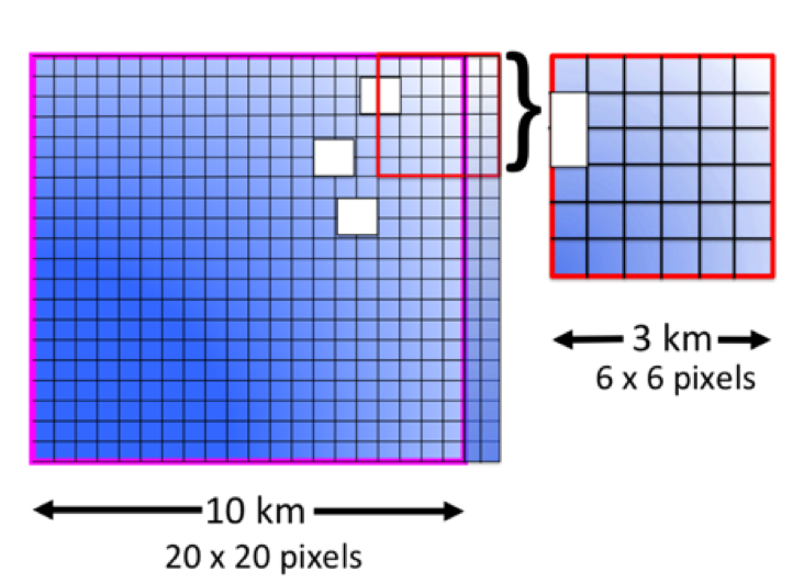
Figure 32:. Illustration of the organization of the MODIS pixels into retrieval boxes for (left) the 10 km product consisting of 20x20 0.5 km pixels within the magenta square and (right) the 3 km product consisting of 6x6 0.5 pixels within the red square. The small blue squares represent the 0.5 km pixels. The white rectangles represent pixels identified as cloudy. The 3 km retrieval box is independent of the 10 km box, and is not a subset. Here it is shown enlarged.
Figure 33 shows a flow chart showing the separate paths for the 10 km and 3 km retrievals. The black boxes running along the center of chart identify processes that are identical in both retrievals. The inputs are identical, as are the masking procedures. The exact same 0.5 km pixels identified as cloud, sediment etc. in the 10 km algorithm are identified as cloud, sediment etc. in the 3 km algorithm. The difference is in how the two algorithms make use of these 0.5 km designations. Once the 3 km algorithm has identified the pixels suitable for retrieval and decided that a sufficient number of these pixels remain, the spectral reflectances are averaged and the inversion continues exactly the same as in the 10 km algorithm. The same assumptions are used, the same look up tables, the same numerical inversion and the same criteria to determine a good fit.
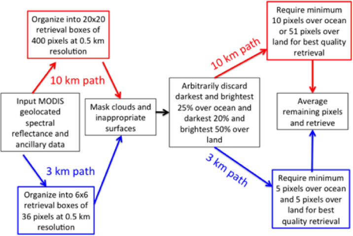
Figure 33: Flowchart illustrating the different paths of the 10 km (red) and 3 km (blue) retrievals. The procedures appearing in the black outlined boxes are common to both algorithms
In the 3 km retrieval the 0.5 km pixels are arranged in retrieval boxes of 6x6 arrays of 36 pixels. Note that in the 3 km retrieval box, the exact same pixels identified as cloudy in the 10 km retrieval box (denoted by the white rectangles) are identified as cloudy in the 3 km box. This is because both algorithms apply identical criteria to mask undesirable pixels. The 3 km retrieval applies a similar deselection of pixels at the darkest and brightest ends of the distribution: 25% and 25% over ocean, and 20% and 50% over land. Once these darkest and brightest pixels are discarded, the algorithm averages the remaining pixels to represent conditions in the 3 km retrieval box. The algorithm requires a minimum of 5 pixels at 0.86 µm over ocean with at least 12 pixels distributed over the other five channels and 5 pixels are required over land in order to continue and make a retrieval. This is actually a more stringent requirement for ocean (14% of 36), than what is required by the 10 km retrieval (2.5%) for the best quality retrieval. The requirement over land is about the same in the 3 km retrieval as it is in the 10 km retrieval (14% and 13%, respectively).
7.2 Granules comparing 10 km and 3 km aerosol products
In Figures 34-37, we show examples from 15 July 2008 and from 12 January 2010 that illustrate the new 3 km product and how it differs from the 10 km product applied to exactly the same input data.

Figure 34: Aerosol optical depth at 550 nm retrieved from the 15 July 2010 Aqua-MODIS radiances using the Collection 6 MODIS Dark Target aerosol algorithm. Left: the product at 10 km resolution. Right: the product at 3 km resolution. This is a moderate dust event over the Mediterranean Sea off the costs of Tunisia and Libya. The 3 km retrieval produces values closer to the coastline and to the islands.
Figure 34 compares the 10 km and 3km ocean retrievals over the Mediterranean Sea off the coast of Tunisia and Libya during a moderate dust event. The two resolution products produce almost the exact same aerosol field with the same gradient and same magnitude aerosol optical depth. This is because the two algorithms are essentially the same. The only difference is that the finer resolution product is able to make retrievals closer to the small islands in the image. We find that this is typical of the 3 km product. It offers over-ocean retrievals closer to land, nearer to islands and within narrow waterways and estuaries.
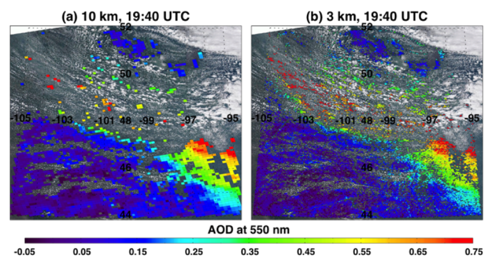
Figure 35: 10 and 3 Km AOD retrievals for a scene over Canada where the 3 km product better resolves the plume from active wildfires. Note the additional red pixels between the clouds in the upper left corner of the image for the 3 km panel.
Figure 35 illustrates the apparent advantage of the 3 km product to resolve smoke plumes from fires. The fire is a large wild fire burning in Canada. The 10 km product does not capture the long narrow smoke plume leading towards the northwest, but the 3 km product does. One of the major advantages of the 3 km product is its ability to better resolve smoke plumes than the 10 km product. Even so, because the cloud identification algorithm in the 3 km product is the same as in the 10 km product, based primarily on spatial variability, the 3 km product still improperly confuses the thickest parts of the smoke plume with a cloud and incorrectly fails to retrieve there.
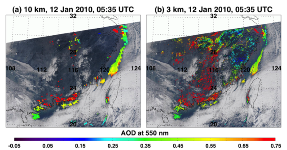
Figure 36: 10 and 3 Km AOD retrievals for a scene from12 January 2010 during a pollution episode in China. Here the 3 km algorithm is able to make retrievals over a much broader region. The AOD interpolated to 0.55 μm from the only AERONET station in the image (Hong Kong PolyU) is 0.38. The 3 km retrieval there is 0.45, while there is no 10 km retrieval available at that spot during this overpass.
Figure 36 demonstrates the potential for different sampling by the two products. The scene is a highly polluted episode over much of southeastern China. Here the 3km algorithm makes retrievals over a broad area, while the 10 km algorithm finds few opportunities to retrieve. The few places of overlap result in similar values of aerosol optical depth. The only AERONET station in the image is at Hong Kong PolyU (22 18 N, 114 11 E), which reports a collocated AOD interpolated to 0.55 μm at MODIS over- pass time of 0.38. The 10 km algorithm does not produce a retrieval at this station, but the 3 km algorithm does, producing an AOD of 0.45, a reasonable match.
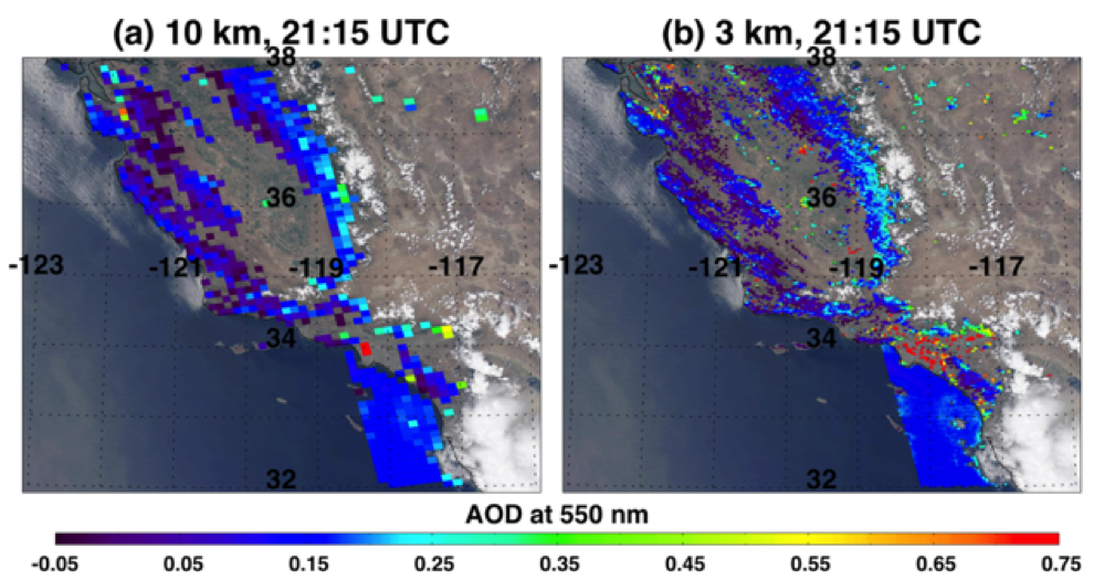
Figure 37: 10 and 3 Km AOD retrieval comparison over California where the 3 km product introduceswidespread artificial noise over an urban area that the 10 km product better confines. There were no collocations with AERONET for this image.
Figure 37 illustrates a potential drawback to using the 3 km product. In this retrieval over the highly urbanized surface of Los Angeles and environs, the surface is incompatible with the current version of the Dark Target retrieval. The pixel selection process of the 10 km algorithm is able to recognize this incompatibility and makes only two retrievals over Los Angeles. However, the 3 km product does retrieve all through the area, and the result is a scattering of retrieved AOD > 0.8 over the region. Although there is no ground truth to determine whether these points are accurate high AOD situations or noisy artifacts of the retrieval, it is highly likely that they are artifacts that the 3 km retrieval fails to avoid. Although the results of the 3 km product mirror the 10 km retrievals, we do find an increase of noisy artifacts in the finer resolution product. This occurs most frequently over urban surfaces, a type of location of significant interest to the air quality community.
7.3 Provisional evaluation of 10 and 3 km products with AERONET and MAN
The six months of test data (January and July 2003, 2008 and 2010) were collocated with Level 2.0 AERONET observations to test the accuracy of the retrievals. For the 10 km retrievals, we use the Petrenko et al. (2012) protocol for collocations, described in section 5.3. Briefly, a collocation is the spatio-temporal average of all AERONET AOD measurements within ±30 min of MODIS overpass and the spatial average of all MODIS 3 km retrievals within a 7.5 km radius around the AERONET station, requiring at least 2 AERONET measurements, and 20% of possible MODIS pixels within the 7.5 km radius. At nadir, the 7.5 km radius can encompass roughly 25 MODIS retrieval boxes, each at 3 km; however, at swath edge, the 7.5 km radius will only encompass 5 retrieval boxes. Therefore, the 20% MODIS retrieval requirement would be at least 5 out of 25 possible retrievals at nadir, but only 1 out of a possible 5 retrieval boxes towards the scan edge. We add the additional restriction of requiring at least 2 retrievals, so that at edge of scan the procedure requires 40% of the area covered to be included in the validation database. Only high quality pixels are included in the collocations. For the 3 km product, we continue to use the same QAC recommendations as the 10 km product (QA = 3 over land and QA > 0 over ocean ). The 10 km product is collocated with AERONET in a similar matter, except that the spatial averaging radius is 25 km, which still encompasses 25 possible MODIS pixels.
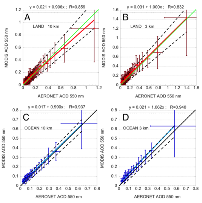
Figure 38: Binned scatter plots of MODIS AOD at 550 nm against AERONET observed AOD. A. MODIS 10 km product over land. B. MODIS 3 km product over land. C. MODIS 10 km product over ocean. D. MODIS 3 km product over ocean. The green(A,B) or black (C,D) line is the 1 : 1 line. The red (A,B) or dark blue (C,D) line is the linear regression through the full database of collocations for 10 km and 3 km, respectively. The dashed lines represent expected error of the MODIS 10 km retrieval. The range of the axes in each plot are different.
Figure 38a shows the binned scatter plots from six months of collocations for land. There are 3252 collocations at 10 km and 2928 at 3 km. The data were sorted according to AERONET AOD and bins designated for every 50 collocations. The mean and standard deviation of both the AERONET and MODIS AODs were calculated. The mean values for each bin are plotted and the error bars indicate ±1 standard deviation. The red line represents the linear regression calculated for the full data set of approximately 3000 collocations and not the roughly 60 bins plotted in the figure. The dashed lines indicate the “expected error” (Levy et al., 2010, Levy et al., 2013). For land the expected error associated with the 10 Km product is
AOD = ±0.05 ± 0.15 AOD (49)
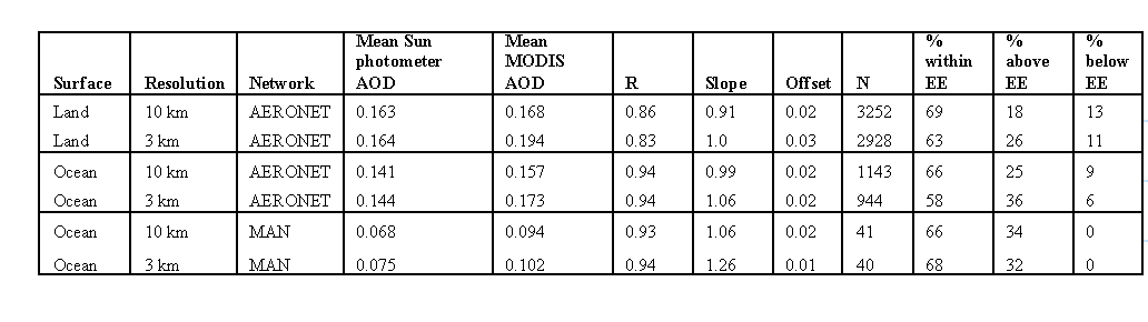
Table 11 provides the mean AOD of each data set, the correlation coefficient, the regression statistics and the number of MODIS retrievals that fall within expected error, fall above the expected error bound (the upper dashed line) and fall below the expected error bound (the lower dashed line in Fig.38a).
Figure 38b shows similar binned scatter plots for the ocean retrieval. There are fewer ocean collocations, 1143 at 10 km and 944 at 3 km. Because AERONET stations are generally on land, the 10 km retrieval with its longer radius will intercept more ocean retrievals than the 3 km retrieval with only a 7.5 km radius. The expected error for ocean is
AOD = ±0.03 ± 0.05 AOD (50)
These figures show the defined expectations associated with this data set with most retrievals falling within expected error (69 % over land and 66 % over ocean). Correlations are high (0.86 over land and 0.94 over ocean) and most retrievals and the linear regression fall close to the 1 : 1 line. The land retrieval does show a positive bias of ∼ 0.005 and the ocean ∼ 0.016, but these are well-within expected uncertainties. Considering the positive high bias and the changed asymmetrical EE bounds over ocean for the 10 km ocean product, we may consider changing the EE over ocean for the 3 km product as well after further evaluation.
Table 11. Parameters from MODIS-AERONET collocation validation: means of each data set, correlation coefficient, regression slope and offset, number of collocations, percent within expected error, percent above expected error and percent below expected error for 10 km and 3 km products separated into land and ocean retrievals. The last rows show MODIS-MAN collocations over ocean.
The 3 km product is also highly correlated to AERONET observations and most of the 3 km retrievals fall within the expected error bounds. However, the 3 km product matches AERONET less well than does the 10 km MODIS product. The most obvious degradation of accuracy between the 3 km and 10 km products is over ocean where the finer resolution product has developed a positive bias of almost 0.03 with only 58 % of retrievals falling within the expected error bounds. The land retrieval has also significantly increased its positive bias against AERONET at finer resolution. In addition to the increased bias, the 3 km land product introduces additional noise at low AOD. This can be seen in the degradation of the correlation coefficient in Table 11.
Because AERONET stations used in the ocean validation collocations are limited to coastal and island stations they do not provide adequate sampling over the open ocean where most of the ocean retrievals take place. The Maritime Aerosol Network is a relatively new network under the AERONET umbrella that offers quality-assured AOD measurements from ships of opportunity over the open ocean (Smirnov et al., 2009). We identified collocations between the MAN AOD and the Aqua-MODIS 10km and 3 km retrievals during the six months of this test data set. A collocation was defined using the same spatial averaging and minimum number of MODIS retrieval criteria as with a MODIS-AERONET collocation. Only ocean retrievals with a QA ≥1 are included in the collocation. Because of the requirement that there be at least 2 or 20 % of available retrievals within a 7.5 km radius for the 3 km product and a 25 km radius for the 10 km product, the two sets of collocations do not necessarily contain the same points. In our sets of MAN-MODIS collocations there are 40 collocations at 3 km and 41 collocations at 10 km, of which 30 are common to both resolutions and 10 and 11 are unique for each resolution, respectively. The AERONET collocation exercise also results in differently sampled data sets, but the results of this different sampling is much more
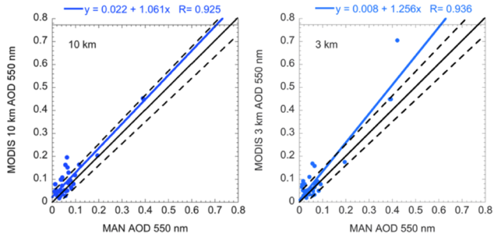
Figure 39: Scatter plot of MODIS 10 km and 3 km retrievals of AOD at 550 nm plotted against collocated data from the Maritime Aerosol Network (MAN). At 10 km and 3 km, 41 and 40 collocations were identified, respectively, in the 6 months undergoing analysis.
The results of the MODIS-MAN collocations are shown in Figure 39. Most MAN collocations occurred in very clean environments with the exception of 3 points (only 2 at 10 km) that occurred in the tropical Atlantic in the dust belt and a moderate value near AOD ∼ 0.2 from the Hudson Bay that appears to be wildfire smoke. The highest AOD collocation in the 3 km data set (9 July 2008 from the dust belt of the Atlantic Ocean with MODIS AOD = 0.67) does not appear in the 10 km database. Most of the MODIS 3 km points agree with the MAN observations to within expectations. The regression and correlation statistics are given in Table 11 but because of the outlying dust point in the 3 km set, these statistics are not robust descriptions of the bulk of the observations. For example while the mean AODs of the MAN and MODIS populations are 0.075 and 0.102, respectively, the medians are 0.047 and 0.061, respectively. The 40 and 41 points are inadequate to fully represent the relationship between MODIS 3 km retrievals over the wide variety of conditions experienced over the world’s oceans. They are shown here to supplement the data set of the AERONET coastal and island sites which is inadequate to provide comparison information over open ocean. Together the available ocean validation does suggest, without firm proof, that the ocean 3 km retrieval will approach similar levels of uncertainty as the well-studied ocean 10 km product, but introduce some additional noise.