The MODIS data files are made available as 5-minute segements from each orbit which are called ‘granules’. Each granule covers an area of about 2030 km along the orbital path and 2330 km (swath width) perpendicular to the oribital path.

	The animation at left illustrates the relative size and shape of the MODIS granules for a single orbit. Global coverage is obtained each day except for small gaps near the equator. Note that the locations of the granules change each day in conjunction with the changing location of the satellite's 16 day orbial cycle.
Animation by Jason Li and Paul Hubanks.

The pixels comprising the data files are at a nominal  1 km resolution at nadir view.  Note, that due to spherical geometry, the size of each pixel increases from 1 km at nadir to nearly 2 km at the swath edges. Each input granule is 1354 by 2030 pixels in this ‘1 km’ resolution. Only data from MODIS daytime orbits are considered for retrieval.

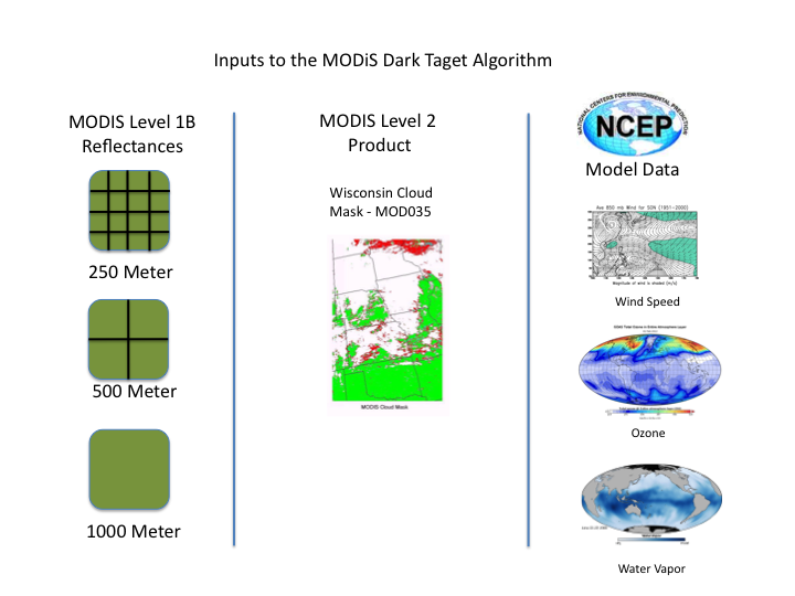
Both the land and ocean aerosol algorithms rely on calibrated, geolocated reflectances (known as ‘Level 1B’ or ‘L1B’) provided by the MODIS Characterization Support Team (MCST). These are identified as products MOD02 and MOD03 for Terra and MYD02 and MYD03 for Aqua.  Note that since the Terra satellite has the longer historical record from here onward our description of the algorithm will refer to the Terra "MOD" files but all Aqua files and products use "MYD" in the file or product name.

The algorithm actually uses L1B reflectances at three resolutions (MOD021KM, MOD02HKM and MOD02QKM for 1 km, 500 m and 250 m resolution channels, respectively). In addition, the MODIS algorithm uses the processed geophysical product (known as ‘Level 2’ or "L2 for short)  MOD35 Wisconsin cloud mask product (Ackerman et al. 1998).  Finally, the algorithm expects ancillary data from NCEP (National Center for Environmental Prediction) analyses, including the (closest to granule time) GDAS1 1°x1° 6 hourly meteorological analysis for water vapor, wind speed and ozone profiles.  In past versions of the product the TOVS (before 2005) or the TOAST (after 2005) 1°x1° daily ozone analysis were used as inputs. Although the algorithm inputs NCEP data, when it is not available at the time of processing climatological data from NCEP is used for first guess water vapor, wind speeds,and ozone profiles.

Processing prior to aerosol retrieval

The aerosol algorithm reads in the required L1B, L2 and ancillary data into memory.  Specifically, for the 10 km retrieval, it reads one scan line at a time, where each scan is made up of ten 1km pixels along track. The 1354 swath pixels are also collected into ten pixel boxes, so that there are 135 ’10 km’ boxes in a swath. Each of these boxes is separately considered for aerosol retrieval.

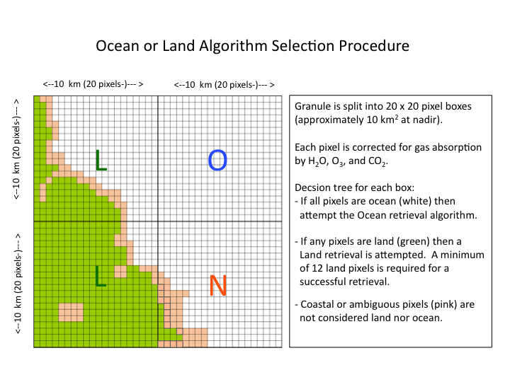
Note that each 10 km box contains 10 x 10 = 100 ‘1 km’ pixels and 20 x 20 = 400 ‘500 m’ pixels. Again note that these sizes refer to the nadir view.  At the scan edges the number of pixels in each box remains the same, but the area encompassed in each box will be double the area encompassed at nadir.

Reflectances in all seven MODIS-aerosol channels, plus the 1.38 µm channel are corrected for water vapor, ozone and carbon dioxide. In addition to the cloud mask, the M?D03 geolocation product also classifies each pixel as ‘land’, ‘ephemeral water’, ‘coastal’, ‘shallow inland water’, ‘deep inland water’, ‘shallow ocean’, ‘moderate ocean’ or ‘deep ocean’.  If all pixels in the 10 km box are considered water (‘deep inland water’, ‘shallow ocean’, ‘moderate ocean’ or ‘deep ocean’), the algorithm proceeds with the over-ocean retrieval. However, if any pixel is considered non-water, then it proceeds with the over-land algorithm. If more than 50% of the pixels with a box are classified as ‘ephemeral water’, ‘coastal’, or ‘shallow inland water’, the algorithm will proceed with the land algorithm, but the retrieval will be assigned a low quality.