
Aerosols, optics and basic retrieval strategy
2.1 Properties of aerosols
Aerosols are a mixture of solid and liquid particles (in a suspension of air) of different sizes, shapes, compositions, and chemical, physical, and thermodynamic properties. They range in size from nanometers to micrometers, spanning from molecular aggregates to cloud droplets. Aerosols between about 0.1 μm and 2.5 μm in radius are of primary interest for climate, precipitation, visibility, and human health studies. Most of these aerosols are found in the troposphere and concentrated toward the Earth’s surface (having a scale height about 2-3 km). Aerosol’s physical and chemical properties are determined by their sources and production processes. Ambient aerosol distributions contain all size ranges although we generally categorize them as belonging to one of two modes. Fine aerosols (radius between 0.1 and 1.0 μm) are formed by coagulation of smaller nuclei (very fine aerosols), or produced directly during incomplete combustion (from biomass-burning or coal power plants). Aerosols larger than about 1.0 μm are known as coarse particles, and are produced primarily from mechanical processes such as erosion of the Earth’s surface. Coarse particles include sea salt and soil dust lifted by winds.
The two aerosol types differ in their spatial distribution and life cycle. Coarse mode particles are usually few in number but can contain the largest portion of aerosol mass (or volume). Because of their larger size (and mass), coarse particles usually settle out of the atmosphere quickly and tend to be concentrated close to their sources. However, convection may lift them into prevailing winds, where they can be transported far from their source. Fine mode, also known as accumulation mode, aerosols have the longest residence time in the atmosphere (days to weeks) because they neither efficiently settle nor coagulate on their own. The fine mode contains the largest portion of aerosol surface area, and therefore the greatest ability to scatter solar radiation. We loosely define the fine aerosol weighting (FW or η) as the ratio of fine aerosol to the total aerosol X, but the exact definition for FW depends on the quantity represented by X (e.g. total mass, total AOD, etc.).
Many aerosols are hygroscopic, meaning that they have the ability to absorb water vapor and thus become involved in cloud processes and the hydrologic cycle. For most fine mode (accumulation-sized) aerosols, the residence time is on the same order as water vapor in the atmosphere, usually about four to fourteen days. Generally, more hygroscopic aerosols (known as hydrophilic, e.g., sulfate or sea salt) are spherical in shape, whereas those less hygroscopic (e.g., hydrophobic, e.g., soot or dust) tend to be non-spherical. Non-spherical aerosols may be clumplike (soot) or crystalline (certain dusts). Larger aerosols usually have shorter residence times (days to hours) due to dry deposition.
For the purposes of aerosol retrieval from satellite, we have to make some assumptions about typical aerosol size distributions and optical properties. We start with basic definitions.
2.1.1 Aerosol size distribution
Because aerosols in nature are not monodisperse, we describe with particle size distributions (PSD) expressed as functions of radius r or diameter D=2r. Although the in-situ community commonly defines in terms of diameter, we typically define in terms of radius. These PSDs may be in terms of number (e.g., nPSD as n(r) ), cross-sectional area (aPSD as ar=πr2 ) or volume (vPSD as v(r)=43πr3. PSD can also be defined via mass, where mass and volume are interchangeable if the particle’s density (mass per volume) is constant. Of course, since radius/diameter are both related to area and volume, the nPSD, aPSD and vPSD are also related. Furthermore, knowing that our size distributions cover orders of magnitude, let’s define our xPSDs (x=n, a, or v) in terms of logged radius (lnr)
Let us start with considering N0 as the total number of particles in the nPSD
\(N_0=\int_{r_{min}}^{r_{max}}{\frac{\mathrm{d}N}{\mathrm{d}\ln{r}}\mathrm{d} \ln{r}}\) (1)
where dN is the number of particles per infinitesimal size “bin” (between lnr and lnr+dlnr). Note that if N0=1 , then dN is the fraction of the particles associated with each size bin. Similarly, one can define the total cross-sectional area and volume (A0 and V0 ) are:
\( A_0=\pi\int_{r_{min}}^{r_{max}}{r^2\frac{\mathrm{d} N}{\mathrm{d}\ln{r}}\mathrm{d} \ln{r}}=\int_{r_{min}}^{r_{max}}{\frac{\mathrm{d}A}{\mathrm{d}\ln{r}}\mathrm{d} \ln{r}}\) (2)
\(V_0=\frac{4\pi}{3}\int_{r_{min}}^{r_{max}}{r^3\frac{\mathrm{d} N}{\mathrm{d}\ln{r}}\mathrm{d} \ln{r}}=\int_{r_{min}}^{r_{max}}{\frac{\mathrm{d}V}{\mathrm{d}\ln{r}}\mathrm{d} \ln{r}}\) (3)
where again, one can normalize to A0=1 or V0=1 (fraction of area or volume in a bin).
For any xPSD (e.g., x=n, a, or v), the mean (arithmetic average) log radius is defined by \({\bar{r}}_x\) :
\({\bar{r}}_x=\frac{1}{X_0}\int_{r_{min}}^{r_{max}}{\ln{r}\frac{\mathrm{d} X}{\mathrm{d}\ln{r}}\mathrm{d} \ln{r}} \) (4)
and standard deviation by σ0,x (square root of variance):
\(\sigma_{0,x}=\sqrt{\frac{1}{X_0}\int_{0}^{\infty}{{(r-{\bar{r}}_x)}^2x\left(r\right)\mathrm{d} r}} \) (5)
It is likely that \({\bar{r}}_n\neq{\bar{r}}_a\neq{\bar{r}}_v \) (mean radius for each xPSD is different).
The median, \({\widetilde{r}}_x\ \) is the 50% or middle value:
\(\frac{X_0}{2}=\int_{r=0}^{r={\widetilde{r}}_x}{x\left(r\right)\mathrm{d} r=\ \int_{{r=\widetilde{r}}_x\ }^{r=\infty}{x\left(r\right)\mathrm{d} r}} \) (6)
For the nPSD, we drop the subscripts, so that \(\bar{r}\equiv{\bar{r}}_n , \sigma_0\equiv \sigma_{0,n} and \widetilde{r}\equiv\ {\widetilde{r}}_n\)
The geometric mean and geometric standard deviation \((r_g and S_g)\ \)of the nPSD are defined as
\(r_g=\exp{\left(\frac{1}{N_0}\int_{0}^{\infty}{\ln{r}n\left(r\right)\mathrm{\ d} r}\right)} \) (7)
\(S_g=\exp{\left(\sqrt{\frac{1}{N_0}\int_{0}^{\infty}{\left(\ln{r-\ln{r_g}}\right)^2n\left(r\right)\mathrm{d} r}}\right)} \) (8)
We can describe the shape of the nPSD is the use of moments, where the ith moment is given by
\(m_i=\int_{0}^{\infty}{\left(r-c\right)^in\left(r\right)\mathrm{d} r}\) (9)
where c is a constant. “Raw” moments refer to using c=0. The 0th raw moment m0 is N0 . The mean is the 1st raw moment normalized by
\(m_0 (e.g. \bar{r}=\frac{m_1}{m_0}). \) The central moments are defined via the mean (\(c=\bar{r})\) ). The variance is the 2nd central moment. Note how the 2nd and 3rd raw moments are related to A0 and V0 . (See table XX).
The effective radius re and effective variance ve are cross-sectional area-weightings useful for optics. By weighting each radius by its cross-sectional area A we get:
\(r_e=\frac{\int_{0}^{\infty}{r\ A\ n\left(r\right)\mathrm{d} }r}{\int_{0}^{\infty}{A\ n\left(r\right)\mathrm{d} r}}=\frac{\int_{0}^{\infty}{r\pi r^2n\left(r\right)\mathrm{d} r}}{\int_{0}^{\infty}{\pi r^2n\left(r\right)\mathrm{d} r}}=\frac{\int_{0}^{\infty}{r^3n\left(r\right)\mathrm{d} r}}{\int_{0}^{\infty}{r^2n\left(r\right)\mathrm{d} r}}=\frac{m_3}{m_2}=\frac{3}{4}\frac{V_0}{A_0} \) (10)
\(v_e=\frac{\int_{0}^{\infty}{{(r-r_e)}^2\ A\ n\left(r\right)\mathrm{d} r}}{{r_e}^2\int_{0}^{\infty}{A\ n\left(r\right)\mathrm{d} r}}=\frac{1}{A_0r_e^2}\int_{0}^{\infty}{{(r-r_e)}^2n\left(r\right)\mathrm{d} r} \) (11)
Both \(r_e \ and \ v_e\) can be defined by moments. Higher order moments help describe skewness and additional statistics. The 2nd and 3rd moments of the nPSD are related to the 0th moments of the aPSD and vPSD, respectively.
| Metric | Moment formulas | Lognormal formulas |
|---|---|---|
| Total number density \(N_0\) | \(m_0 \) | \(N_0\) |
| Number mean radius \(\bar{r}\) | \(\frac{m_1}{m_0} \) | \(\frac{1}{N_0}N_0\exp{\mu+\ \frac{\sigma^2}{2})\ }=\ \ \widetilde{r}\exp\frac{\sigma^2}{2})\ \) |
| Variance \(\sigma_0^2\) | \(\frac{m_2}{m_0}-\left(\frac{m_1}{m_0}\right)^2 \) | \({\widetilde{r}}^2\exp{\left({2\sigma}^2\right)\ -}\ {\widetilde{r}}^2\exp{\left(\sigma^2\right)}={\widetilde{r}}^2\exp{\left(\sigma^2\right)}[\exp{\left(\sigma^2\right)-1}]\) |
| Total cross-sectional area density \(A_0\) | \({\pi m}_2\) | \({\pi N}_0\exp{\ (2\mu+\ {2\sigma}^2)\ }=\ {\pi N}_0\ {\widetilde{r}}^2\exp{\left({2\sigma}^2\right)}\) |
| Total volume density \(V_0\) | \({\frac{4}{3}\pi m}_3\) | \({\pi N}_0\exp{(2\mu+\ {2\sigma}^2)\ }=\ {\pi N}_0\ {\widetilde{r}}^2\exp{\left({2\sigma}^2\right)} {\frac{4}{3}\pi m}_3 \) |
| Effective radius \(r_e\) | \(\frac{m_3}{m_2}\) | \(\frac{\exp{ (3\mu+\ 4.5\sigma^2)\ }}{\exp{ (2\mu+\ 2\sigma^2)\ }}=\widetilde{r}\exp (2.5\sigma^2)\) |
| Effective variance \(v_e\) | \(\frac{m_2m_4}{{m_3}^2}-1 \) | \(exp\left(\sigma^2\right)-1\) |
| Number median radiance \(\widetilde{r}\) | \(exp(\mu)-1\) | |
| Area median radiance \(\widetilde{r}_a\) | \(\exp{(\mu_a)}=\exp{\left(\mu+{2\sigma}^2\right)} = \widetilde{r}\exp (2\sigma^2) \) | |
| Volume median radiance \(\widetilde{r}_v \) | \(\exp{{(\mu}_v)}=\exp{\left(\mu+{3\sigma}^2\right)} = \widetilde{r}\exp (3\sigma^2)\) | |
| Area-weighted mean radiance \(\bar{r}_a\) | \(\frac{m_3}{m_2}\) | \({\widetilde{r}}_a\exp{\left(\frac{1}{2}\sigma^2\right)}=\widetilde{r}\exp (\frac{5}{2}\sigma^2)\) |
| Volume-weighted mean radiance \({\bar {r}}_v\) | \(\frac{m_4}{m_3}\) | \({\widetilde{r}}_v\exp{\left(\frac{1}{2}\sigma^2\right)}=\widetilde{r}\exp(\frac{7}{2}\sigma^2)\) |
Of course, PSDs can be generic, but it is common for remote sensing algorithms to assume a mathematical function for the PSD. Because particle size may cover several orders of magnitude, a Normal (Gaussian) Distribution (ND) may not be useful. The literature commonly uses lognormal (LND), Gamma (GD), and Modified Gamma (MGD), with the LND the most common for our remote sensing. The LND is extremely convenient, because we can define nPSD in terms of \(l=\ln{r}\). The total number of particles \(N_0\) is the same whether in r space or l space, e.g.,
\(N_0=\int_{r=0}^{r=\infty}{n\left(r\right)\mathrm{d} r=}\int_{0}^{\infty}{\frac{\mathrm{d}N\left(r\right)}{\mathrm{d}r}\mathrm{d} r=}\int_{\ln{r}=-\infty}^{\ln{r}=\infty}{\frac{\mathrm{d}N\left(\ln{r}\right)}{\mathrm{d}\ln{r}}\mathrm{d} \ln{r}=}\int_{l=-\infty}^{l=\infty}{n_l\left(l\right)\mathrm{d} l}\) (12)
In other words,
\(n_l\left(l\right)=\frac{dN(l)}{dl}=\frac{dN(\ln{r})}{d\ln{r}}=\frac{N_0}{\sqrt{2\pi}}\frac{1}{\sigma\ }\exp{\left[-\frac{\left(l-\mu\right)^2}{{2\sigma\ }^2}\right]}\) (13)
where \(\mu\) and \(\sigma\) are the standard deviation of \(l\) between
\(\mu=\frac{1}{N_0\ }\int_{l=-\infty}^{l=\infty}{l\ n_l\left(l\right)\mathrm{d} l}\) (14)
\(\sigma=\sqrt{\frac{1}{N_0\ }\int_{-\infty}^{\infty}{{(l-\mu)}^2n_l\left(l\right)\mathrm{d} l}}\) (15)
By noting the similarities of Eq (14) with Eq (8) and Eq (15) with Eq (9) we see that
\(\mu=\ln{r_g} \ and\)
\(\sigma=\ln{S_g\equiv}\sigma_g\) (16)
In other words, the arithmetic mean and standard deviation in log-size space are equal to the geometric mean and standard deviation in size space!
If we note that:
\(\frac{\mathrm{d}l}{\mathrm{d}r}=\frac{1}{r}\) (17)
then in terms of diameter rather than log-diameter, we can write
\(n\left(r\right)=\ \frac{dN(r)}{dr}=\frac{\mathrm{d} N(l)}{\mathrm{d}l}\frac{\mathrm{d} l}{\mathrm{d}r}=n_l\left(l\right)\frac{\mathrm{d} l}{\mathrm{d}r}=\frac{N_0}{\sqrt{2\pi}}\frac{1}{\sigma}\frac{\ 1}{r}\exp{\left[-\frac{\left(\ln{(r)}-\mu\right)^2}{{2\sigma}^2}\right]}\) (18)
Or in terms of geometric means and standard deviations,
\(n\left(r\right)=\frac{N_0}{\sqrt{2\pi}}\frac{1}{\ln(S_g)}\frac{\ 1}{r}\exp{\left[-\frac{\left(\ln{(r})-\ln{{(r}_g)}\right)^2}{2\ln^2{\left(S_g\right)}}\right]} \) (19)
We must be careful about the use of σ vs Sg because the aerosol community uses both! Typical aerosol distributions have Sg in the range 1.5 - 2.0, with σ in the range of 0.4 - 0.7. We choose to use σ for convenience. Furthermore, the mean (average), median (50%) and the mode (peak) in log-space all have the same values \((\mu=\widetilde{l}=l_m)\). And as the midpoint of the distribution, the median in log-space is identical to the log of the median in linear space, (e.g.,\(\widetilde{l}=ln\widetilde{r}\)). This also means geometric mean radius \(r_g\) is the same as the median radius\(\widetilde{r}\) ! The mode size is related to the median by\(\ln{r_M}=\ln{\widetilde{r}}-\ \sigma^2\) . For a LND, one can show that geometric standard deviations for the nPSD, aPSD, and vPSD are equal!
2.1.2 Aerosol optical properties
Aerosols are important actors on the Earth’s climate and radiation due to their size. Particles most strongly affect the radiation field when their size is most similar to the wavelength of the radiation [e.g. Chandresekhar, 1950]. Aerosols in the fine mode (0.1 to 1.0 μm) are similar in size to the wavelengths of solar radiation within the atmosphere, and are also the largest contributors to aerosol surface area. Radiation incident on aerosols may be absorbed, reflected or transmitted, depending on the size, chemical composition (complex refractive index, m+ik) and orientation (if non-spherical) of the aerosol particles. Scattering and absorption quantities may be represented as functions of path distance (the scattering/absorption coefficients, βsca/βabs, each in units of “per length”), number (the scattering/absorption cross sections, σsca/σabs, each in units of area) or mass (the scattering/absorption mass coefficients,Bsca/Babs, each in units of area per mass). The conventions on the use of symbols is inconsistent in the literature. For this work we define extinction following Liou [2002]: Extinction (coefficient/cross section/mass coefficient) is the sum of the appropriate absorption and scattering (coefficients/cross sections/mass coefficients), e.g.,
 (11)
(11)
for the cross sections (σ here refers to a different parameter than was used in section 2.1.1). These properties define the amount of radiation ‘lost’ from the radiation field, per unit of material loading, in the beam direction. Note all of the parameters are dependent on the wavelength λ. The ratio of scattering to extinction (e.g., βsca/βext) is known as the single scattering albedo (SSA or ω0). As most aerosols are weakly absorbing in mid-visible wavelengths (except for those with large concentrations of organic/black carbon), extinction is primarily caused by scattering (ω0 > 0.90 at 0.55 mm). Black or elemental carbon (soot) can have ω0<0.5 [Bond and Bergstrom, 2006] especially near sources. Mineral dusts are unique in that they have a spectral dependence of absorption, such that they absorb more strongly in short visible and UV wavelengths (λ<0.47 mm) than at longer wavelengths.
Properties of extinction (scattering and absorption) can be calculated, and are dependent on the wavelength of radiation, as well as characteristics of the aerosols’ size distribution, chemical composition, and physical shape. For a single spherical aerosol particle, the combination of refractive index), and Mie size parameter, X (relating the ratio of radius to wavelength, i.e., X=2πr/λ uniquely describe the scattering and extinction properties of the particle.
The scattered photons have an angular pattern, known as the scattering phase function (Pl (Θ)), which is a function of the scattering angle (Θ) and wavelength. In other words, the Mie quantities describe the interaction between an incoming photon and aerosol particle, whether it is displaced, scattered, and towards which direction relative to the incoming path.
For a distribution of aerosol particles, one is concerned with the scattering by all particles within a space (e.g., per volume, per atmospheric column). In general, since the average separation distance between particles is so much greater than particle radius, particles can be considered independently of each other.
Light scattering by aerosols is a function of the wavelength, the aerosol size distribution, and the aerosol composition [Fraser, 1975]. The asymmetry parameter, g, represents the degree of asymmetry of the angular scattering (phase function), and is defined as:
 (12)
(12)
Values of g range from -1 for entirely backscattered light to +1 for entirely forward scattering. For molecular (Rayleigh) scattering, g=0. For aerosols, g typically ranges between 0.6 and 0.7 (mostly forward scattering), with lower values in dry (low relative humidity) conditions [Andrews et al., 2006]. Specifically, g is strongly related to the aerosol size, especially of the accumulation mode.
Comparing the scattering properties at two or more wavelengths provides information about the bulk aerosols’ size. The Ångstrom exponent (AE or α) relates the spectral dependence of the extinction (or scattering) at two wavelengths, λ1 and λ2:
 (13)
(13)
[Ångstrom, 1929; Eck et al., 1999]. Typically for aerosol, the two wavelengths are defined in the visible or infrared (e.g., 0.47 and either 0.66 or 0.87μm). Smaller aerosol sizes produce higher values of a, such that aerosol distributions considered to be fine aerosol dominated have α ≥ 1.6, whereas those dominated by coarse aerosols have α ≤ 0.6. Quadratic fits to more than two wavelengths, known as modified Ångstrom exponents [O’Neill et al., 2001], can provide additional size information including the relative weighting of fine mode aerosol to the total designated as FW, or η.
The aerosol optical depth (AOD) is the integral of the aerosol extinction coefficient over vertical path from the surface to the top of the atmosphere (TOA), i.e.
 (14)
(14)
where the subscript p represents the contribution from the particles (to be separated from molecular or Rayleigh optical depth). Typically, AOD (at 0.55 μm) range from 0.05 over the remote ocean to 1.0, 2.0 or even 5.0, during episodes of heavy pollution, smoke or dust. Note, that since vertical path is the same regardless of the wavelength, the AE can also be calculated from spectral AOD.
2.2 “Dark-target” retrieval strategy
Aerosol Optical Depth (AOD) is the fundamental parameter in aerosol remote sensing. The simplest way to “measure” AOD using a passive remote sensing technique is with sunphotometry [Volz, 1959]. A sunphotometer views the solar disc through a collimator, and measures the extinction of direct-beam radiation in distinct wavelength bands. The measurement assumes that the radiation has had little or no interaction with the surface or clouds, and that there is minimal (or known) gas absorption in the chosen wavelength λ. In other words, sunphotometry is a basic application of the Beer-Bouguer-Lambert law which relates the attenuation of light to the properties of the media through which it is traveling, in the form of:
 (15)
(15)
where L, is the measured solar radiance, F0, the extra-terrestrial solar irradiance (irradiance outside the atmosphere), d, the ratio of the actual and average Earth/Sun distance, θ0, the solar zenith angle, τt, the total atmospheric optical depth, and m t the total relative optical air mass. The factor τtmt is the only unknown, and it can be further broken down as:
 (16)
(16)
where the superscripts t, R, a and g refer to total, molecular (Rayleigh scattering), aerosol, and gas absorption (variably distributed gases such as H2O, O3, NO2, etc.), where the relative optical air masses of each component differ due to differing vertical distributions. The molecular portions of (16) are primarily dependent upon altitude of the surface target, and thus can be accurately calculated (e.g., Bodhaine et al., [2003]). The gas absorption portion, while varying in vertical profile by component, can also be reasonably estimated. Therefore, since errors are well defined, estimation of AOD (τa, or hereby simplified as τ) is straightforward from a sunphotometer. When made at more than one wavelength, sunphotometers retrieve spectral (wavelength dependent) τ, which in turn can be used to characterize AE, and the relative size of the ambient aerosol [Eck et al., 1999; O’Neill et al., 2003].
Retrieving AOD from a satellite is a more complicated process. For one, the geometry of the sensor/target/satellite light path is such that instead of one, there are two passes through the atmosphere. Instead of measuring extinction (and accurately retrieving AOD), a satellite measures back scattered (reflected) light. The scattered light comes not only from the atmosphere, but also from the surface directly, and through surface/atmosphere interactions. This means that for a satellite aerosol retrieval, we either have to find situations where the surface contribution is negligible, or can be assumed with accuracy. The geometry of the satellite measurement is illustrated in Fig 2, such that θ0, θ and Φ are the solar zenith, target view zenith and relative solar/target relative azimuth angles, respectively. The scattering angle, Θ is:
 (17)
(17)
Note that in the context of satellite observations the Earth’s surface is considered the vantage point when we refer to the ‘sensor’ angles or ‘view’ angles of the satellite target.
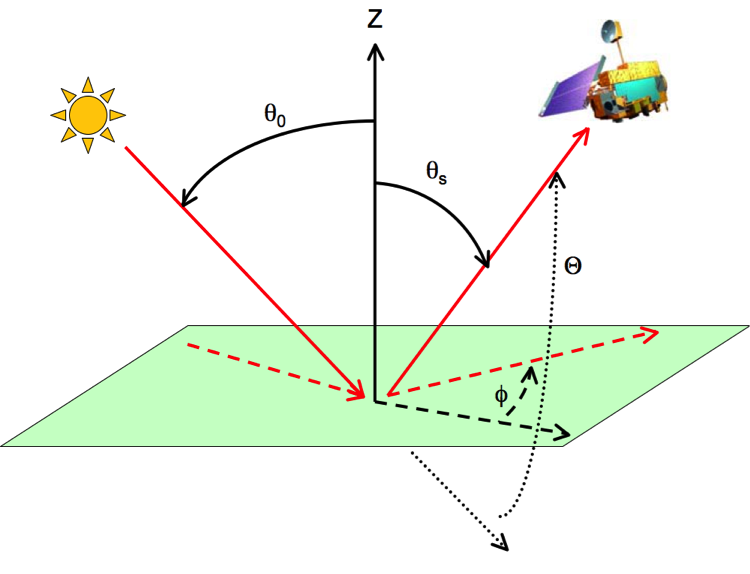
Fig 2: Schematic of sun/surface/satellite remote sensing geometry, defining the angles as viewed from the surface target. The solid lines (and curves) represent solar zenith θo and satellite view zenith θs angles (measured from the zenith, Z). The dashed lines (and curves) represent the relative azimuth angle Φ (measured from the extension of the solar azimuth), and the dotted lines (and curves) represent the scattering angle Θ (measured from the extension of the direct beam). The Terra icon is from the Earth Observatory (http://earthobservatory.nasa.gov).
Since satellite retrieval is primarily a problem of reflected radiation, it is easier to deal with equations in terms of reflectance. The normalized spectral radiance, or reflectance, ρ is defined by
 (18)
(18)
The upward reflectance (normalized solar radiance), at the top of the atmosphere (TOA), is a function of successive orders of radiation interactions within the coupled surface-atmosphere system. It includes scattering of radiation within the atmosphere (the ‘atmospheric path reflectance’), reflection of radiation off the surface that is directly transmitted to the TOA (the ‘surface function’), and reflection of radiation from outside the sensor’s field of view (the ‘environment function’). The environment function is neglected so that to a good approximation:
 (19)
(19)
where ρaλ represents the atmospheric path reflectance, including aerosol and molecular contributions, Tλare the ‘upward (and downward) transmissions’ (direct plus diffuse) defined for zero surface reflectance (reciprocity implied), sλ is the ‘atmospheric backscattering ratio’ (diffuse reflectance of the atmosphere for isotropic light leaving the surface), and ρsλ is ‘surface reflectance’ [Kaufman et al., 1997a], which for now we assume to be Lambertian. The more non-reflective the surface is (a “dark target”), the more one can neglect the 2nd term. In essence the goal of the satellite retrieval process is to first isolate the atmospheric path reflectance then determine the portion that is contributed by aerosol (e.g. the aerosol path reflectance). Fig. 3 demonstrates the spectral response of aerosol scattering for a number of idealized aerosol types.
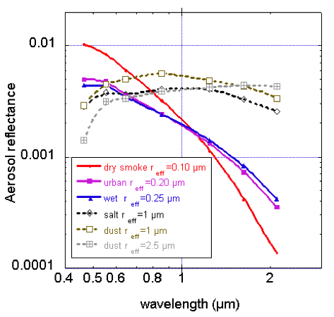
Fig. 3: Spectral dependence of aerosol reflectance for selected aerosol types viewed from the top of the atmosphere (for some arbitrary AOD). Aerosol reflectance depends on single scattering albedo, phase function and total aerosol loading. (Figure from the work of Yoram Kaufman).
Finally, the path reflectance can be broken down into its components, so that the total path reflectance (for a given wavelength) is the sum of each aerosol mode’s fractional contribution. If, say, there are two modes (a fine and a coarse mode), then the total path reflectance is the sum of the two contributions, weighted by the fine mode fraction (η).
 (20)
(20)
Except for the surface reflectance, each term on the right hand side of Eq. (19) is a function of the atmospheric state, which includes molecular and gas terms, as well as the aerosol (spectral τ) we are trying to derive.
If we assume that:
a) our satellite is observing only in atmospheric windows, so that gas absorption is negligible and
b) that we have properties of aerosol size distribution (e.g. rg, V0 and σ for one or more modes) and complex refractive indices (m+ik) for these modes
then we can calculate the properties of aerosol scattering/extinction and phase functions.
Next, we assume the vertical profile for the aerosol and molecular scatterings, so that we can use radiative transfer (RT) code to simulate TOA path radiance (ra) for any wavelength, along with atmospheric transmissions (Tλup and Tλdown) and the backscattering ratio (s). This is the basis for a lookup table (LUT) that can be expanded to represent any number of angles (combinations of θ0,θ and Φ), aerosol types (size + refractive index), and aerosol loadings (τ).
In order to solve Eq.(19) we use calculated LUTs for a fine-dominated aerosol model and a coarse-dominated aerosol as well as the following assumptions:
- The surface reflectance ρs is “small” or can be accurately characterized in three or more wavelengths.
- We can iterate the LUTs to find solutions of fine and coarse type aerosols that, coupled with surface reflectance assumptions, add up to ρ*.
- The best solution is the one that leads to a “minimum” difference between estimated ρ* and ρm (measured spectral reflectance).
In other words, if we assume that we can somehow account for the surface reflectance, we can iterate through the LUT to determine the aerosol conditions that add up to ρ* and best mimic the sensor-observed spectral reflectance ρmλ. Of course, the challenge lies in making the most appropriate assumptions about both the surface and atmospheric contributions. A second issue is the inversion/iteration, and how to ensure that the aerosol solution is in fact an appropriate and physically relevant solution. The solutions, thus include the total AOD (loading), and the relative contributions of fine and coarse aerosol types (η).
A major problem related to any aerosol retrieval is deciding which surface targets to retrieve over. The dark-target aerosol retrieval is a clear-sky algorithm, and there are clouds everywhere. Therefore cloud masking and pixel selection strategies are important components to this aerosol retrieval.
Finally, since ocean and land surfaces have such different optical properties, the strategies for retrieving AOD and η (ETA) differ over each surface. In fact, the DT algorithm is actually two separate algorithms. The details of the ocean and land algorithms are given in later sections, but first we discuss the sensors, their spectral characteristics, and the environment for which we run the aerosol retrieval algorithm.