6. Algorithm description: ocean

6.1 Strategy

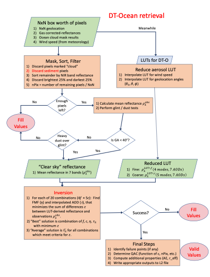
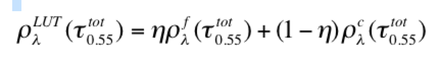
Let us assume that from the Main core, we have received an N x N worth of gas-corrected pixels, \(\rho_\lambda\)^L1B along with the geolocation, cloud mask results (assuming the entire N x N box is ocean), and the ancillary wind speed information. The mechanics of the ocean algorithm are illustrated in figure 6-1. The basic strategy of the dark target aerosol retrieval over the ocean (DT-O) is described in in Tanré et al. [1997], Levy et al.  [2003], Remer et al. [2005] with the dynamic wind speed addition explained in Kleidman et al. [2012]. It follows the DT strategy presented in Section 2.2, in that one fine “f” and one coarse “c” aerosol model can be combined with FMW ( \(\eta\) ) to represent the ambient aerosol properties and TOA spectral reflectance (Eq. 2-27.; rewritten here), 

          Equation 6-1

Spectral reflectance from the LUT is compared with MODIS-measured spectral reflectance to find the ‘best’ (least-squares) fit. The best fit, or an ‘average’ of a set of the best fits is used as the solution to the inversion. Although the core inversion remains similar to the process described in Tanré, et al. (1997), and updates including sediment masking and the special handling of heavy dust including dust retrievals over glint included in ATBD-09, minor updates to masking of clouds and the inclusions of multiple wind speed look-up tables are new. In this section, we describe the over-ocean LUTs, the cloud masking and pixel selection logic, the retrieval strategy details, and over-ocean product description.

 

6.2   LUTs for DT Ocean

   6.2.1  Aerosol Models

The aerosol optical models for DT-O are derived mainly from data gleaned from sun/sky photometers (e.g. AERONET; Holben et al., [1998]), and from analysis of errors in the products from previous versions of the algorithm. For DT in general, there are four fine modes and five coarse modes, with spectral refractive indices and lognormal size parameters computed via a Mie code. Table 6 -1 to Table 6-4 describe spectral properties of the aerosol modes for the exact MODIS wavelengths (Table 3-2.), for unit AOD =1.0 (at 0.55 mm).  Other sensors will have similar spectral properties, although different exact values at their respective wavelengths. Figure 6-2 illustrates the properties of 4 fine and 5 coarse modes for the DT-O, plotted at MODIS and VIIRS wavelengths, computed for AOD = 1.0 at 0.55 μm.

Table 6-1 (A): Refractive Indices, Number Median, Standard Deviation and Effective Radius for the aerosol modes used in the MODIS Lookup Table for the ocean algorithm.  Models 1-4 are fine modes and Models 5-9 (table 6-1(B) are coarse modes. All modes listed here are assumed spherical.

F	\(\lambda\)  = blue, green, red, NIR	\(\lambda\) =NIR1	\(\lambda\) =SWIR1	\(\lambda\) =SWIR2	rg	\(\sigma\)	reff	Comments
1	1.45-0.0035i	1.45-0.0035i	1.43-0.01i	1.40-0.005i	0.07	0.40	0.10	Water Soluble
2	1.45-0.0035i	1.45-0.0035i	1.43-0.01i	1.40-0.005i	0.06	0.60	0.15	Water Soluble
3	1.40-0.0020i	1.40-0.0020i	1.39-0.005i	1.36-0.003i	0.08	0.60	0.20	Water Soluble + humidity
4	1.40-0.0020i	1.40-0.0020i	1.39-0.005i	1.36-0.003i	0.10	0.60	0.25	Water Soluble + humidity

Table 6-1 B

C	\(\lambda\) =blue, green, red, NIR	\(\lambda\) =NIR1	\(\lambda\) =SWIR1	\(\lambda\) =SWIR2	rg	\(\sigma\)	reff	Comments
5	1.35-0.001i	1.35-0.001i	1.35-0.001i	1.35-0.001i	0.40	0.60	0.98	Wet sea salt type
6	1.35-0.001i	1.35-0.001i	1.35-0.001i	1.35-0.001i	0.60	0.60	1.48	Wet sea salt type
7	1.35-0.001i	1.35-0.001i	1.35-0.001i	1.35-0.001i	0.80	0.60	1.98	Wet sea salt type
8	1.53-0.003i (blue) 1.53-0.001i (green) 1.53-0.000i (red, NIR)	1.46-0.000i	1.46-0.001i	1.46-0.000i	0.60	0.60	1.48	Dust-like type
9	1.53-0.003i (blue) 1.53-0.001i (green) 1.53-0.000i (red, NIR)	1.46-0.000i	1.46-0.001i	1.46-0.000i	0.50	0.80	2.50	Dust-like type

 

Table 6‑2: Spectral AOD dependence for the nine spherical aerosol modes for MODIS wavelengths. Right two columns are Ångstrom Exponent .

\(\lambda\) (\(\mu\)m) Mode	0.466	0.554	0.645	0.857	1.241	1.628	2.113	AE	0.86  0.55	2.11 0.86
1 F	1.539	1	0.66	0.285	0.086	0.047	0.016		2.877	3.183
2 F	1.305	1	0.764	0.426	0.17	0.081	0.03		1.957	2.927
3 F	1.247	1	0.796	0.481	0.213	0.105	0.042		1.677	2.696
4 F	1.187	1	0.832	0.547	0.269	0.14	0.06		1.385	2.449
5 C	0.966	1	1.022	1.026	0.918	0.764	0.586		-0.058	0.619
6 C	0.967	1	1.033	1.093	1.118	1.058	0.927		-0.204	0.182
7 C	0.977	1	1.026	1.087	1.166	1.179	1.124		-0.191	-0.037
8 C	0.977	1	1.026	1.087	1.185	1.192	1.127		-0.19	-0.04
9 C	0.982	1	1.019	1.059	1.118	1.137	1.126		-0.131	-0.069

Table 6‑3: Spectral Single Scattering Albedos for the nine spherical aerosol modes for MODIS wavelengths 

\(\lambda\) (\(\mu\)m) Mode	0.466	0.554	0.645	0.857	1.241	1.628	2.113
1 F	0.974	0.968	0.961	0.94	0.879	0.541	0.499
2 F	0.978	0.977	0.976	0.97	0.956	0.817	0.822
3 F	0.987	0.986	0.986	0.984	0.978	0.921	0.916
4 F	0.986	0.987	0.987	0.985	0.982	0.94	0.941
5 C	0.978	0.982	0.985	0.989	0.991	0.992	0.993
6 C	0.966	0.972	0.976	0.983	0.988	0.991	0.992
7 C	0.955	0.962	0.967	0.976	0.984	0.988	0.99
8 C	0.901	0.967	1	1	1	0.99	1
9 C	0.867	0.953	1	1	1	0.983	1

 

 

Table 6‑4: Spectral Asymmetry Parameters for the nine spherical aerosol modes for MODIS wavelengths

\(\lambda\) (\(\mu\)m) Mode	0.466	0.554	0.645	0.857	1.241	1.628	2.113
1 F	0.576	0.511	0.447	0.321	0.178	0.105	0.063
2 F	0.683	0.66	0.635	0.575	0.468	0.369	0.265
3 F	0.735	0.718	0.699	0.651	0.559	0.472	0.372
4 F	0.751	0.74	0.726	0.69	0.618	0.546	0.458
5 C	0.785	0.786	0.789	0.794	0.795	0.787	0.769
6 C	0.795	0.788	0.786	0.787	0.794	0.796	0.792
7 C	0.81	0.8	0.793	0.786	0.788	0.794	0.796
8 C	0.753	0.72	0.697	0.679	0.713	0.72	0.719
9 C	0.78	0.746	0.723	0.706	0.722	0.722	0.715

 

 

 

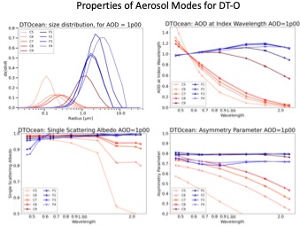
The DT-O LUT employs the Ahmad and Fraser (1981) vector radiative transfer (AFRT) code to simulate TOA reflectance for a coupled ocean/atmosphere. AFRT includes toggles for whether to include polarization (turned on), trace gas coupling (turned off) and pseudospherical atmosphere (turned on). AFRT includes an internal Mie code (for calculating scattering properties of spherical particles) but can be set up to use external calculations of scattering properties (if non-spherical). For spherical modes 1F to 9C all Mie calculations are performed internally. 

6.2.2. Reflectance-versus-Aerosol LUT

The spectral reflectance at the satellite level is the coupled combination of radiation from the surface and the atmosphere. The ocean surface calculation includes sun glint reflection off the surface waves [Cox and Munk, 1954], reflection by foam and whitecaps [Koepke, 1984] and Lambertian reflectance from underwater scattering (sediments, chlorophyll, etc). The LUT includes simulations for four wind speeds, 2 m/s, 6 m/s, 10 m/s, and 14 m/s, having foam fractions of 0.01%, 0.16%, 1% and 3%, respectively (e.g. Monahan and Muircheartaigh, [1980] ). Zero water leaving radiance is assumed for all compared wavelengths, except for the green, where a fixed reflectance of 0.005 is used. The atmospheric contribution includes multiple scattering by gas and aerosol, as well as reflection of the atmosphere by the sea surface. Central wavelengths, Rayleigh optical depths and molecular depolarization factors (also known as King factors) are prescribed in the AFRT, based on the exact characteristics of the sensor’s wavelength bands. 

Thus, TOA spectral reflectance is computed for each of the nine spherical aerosol models (combined with Rayleigh and surface) described in the Table 6‑1. Six values of total aerosol loading (AOD at 0.55 μm, denoted as t number of AOD) are considered for each mode, ranging from a pure molecular (Rayleigh) atmosphere (\(\tau\) 0.0) to a highly turbid atmosphere (\(\tau\)  = 3.0), with intermediate values of 0.2, 0.5, 1.0 and 2.0.  For each model and aerosol optical depth at 0.55 μm, the associated aerosol optical depths are stored for all the sensor’s seven wavelengths, including the blue, which is not used in the least squares fit to spectral reflectance. Also stored are aerosol optical depth values for the sensor’s green channel, which may or may not be the same as the reference wavelength of 0.55 µm. Computations are performed for combinations of 11 solar zenith angles (6°, 12°, 24°, 36°, 48°, 54°, 60°, 66°, 72°, 78° and 84°), 16 satellite view zenith angles (0° to 72°, increments of 6°) and 16 relative sun/satellite azimuth angles (0° to 180°, increments of 12°) for a total of 2816 angular combinations. Again, note that scattering and LUT calculations are specific for a given sensor’s wavelength band, however always normalized to AOD = 1.0 at 0.55 μm.  Also note that for sensors that do not include a particular band (e.g., no NIR1 on ABI or AHI), placeholders are included so that the LUT will always be indexed for 7 wavelengths. Let us denote the spectral reflectance in the LUT as (\rho_\lambda\)^LUT, where v, j, , are indices for windspeed, aerosol model, aerosol loading (defined by AOD at 0.55 mm), and angles. During the retrieval, this LUT spectral reflectance is interpolated to represent the actual wind speed (provided by ancillary information) and angles. 

Ocean Glint and Internal Consistency:

The ocean algorithm was designed to retrieve only over dark ocean (i.e. away from glint). There is a special case when we retrieve over glint which is described below. The algorithm calculates the glint angle, which denotes the angle of reflection, compared with the specular reflection angle. The glint angle is defined as

  Θ_glint=cos^–1((cosθ_scosθ_v)+(sinθ_ssinθ_vcosΦ))                            (25)

where θ_s, θ_v, and Φ are the solar zenith, the satellite zenith and the relative azimuth angles (between the sun and satellite), respectively. Note that Fresnel reflection corresponds to Θ_glint = 0.  If Θ_glint > 40˚, we can avoid glint contamination and proceed with the retrieval. The algorithm performs several consistency checks of the spectral reflectances. Depending on the outcome of these consistency checks, the algorithm may either declare the reflectances to be beyond the range necessary for a successful inversion and exit the procedure, or continue onto the inversion after assigning quality flags (Quality Assurance – QA) to each wavelength.

4.4 Retrieval Algorithm

The ocean inversion procedure described in ATBD-96, Levy et al., (2003) and Remer et al., (2005) remains the same for the C6-O algorithm. Following Tanré et al. (1996), we know that the MODIS-measured spectral radiance (0.55 – 2.13 µm) contains almost three pieces of independent information about the aerosol loading and size properties. With some assumptions, the algorithm can derive three parameters: the τ at one wavelength τ^tot_0.55  , the ‘reflectance weighting parameter’ (the over-ocean definition of Fine Weighting - η) at one wavelength (η_λ=0.55 ) and the ‘effective radius’ (r_e), which is the ratio of the 3rd and 2nd moments of the aerosol size distribution. The effective radius is represented by choosing a single ‘fine’ (f) and single ‘coarse’ (c) aerosol mode for weighting with the η parameter. The inversion is based on the look-up table (LUT) of four fine modes and five coarse modes (Table 2).  Although the LUT is defined in terms of a single wavelength of optical thickness, the parameters of each of the single mode models define a unique spectral dependence for that model, which is applied to the retrieved value of , to determine optical thickness at the other reported wavelengths.

The retrieval requires a single fine mode and a single coarse mode. The difficulty is in determining which of the (4 x 5 =) twenty combinations of fine and coarse modes and their relative optical contributions that best mimics the MODIS-observed spectral reflectance. To accomplish this the reflectance from each mode is combined using η as the weighting parameter,

                (26)

 

where is a weighted average reflectance of an atmosphere with a pure fine mode 'f' and optical thickness and the reflectance of an atmosphere with a pure coarse mode 'c' also with the same.  For each of the twenty combinations of one fine mode and one coarse mode, the inversion finds the pair of  and η_0.55  that minimizes the ‘fitting error’ (ε) defined as

 

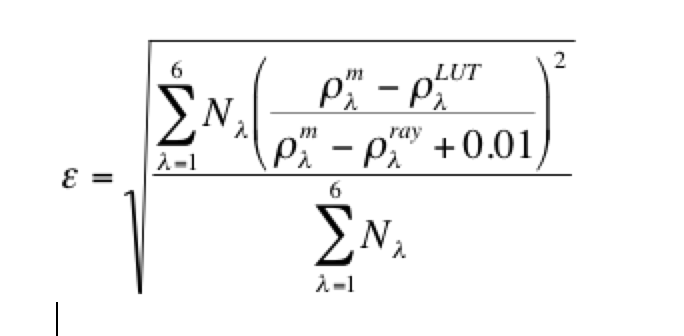                                                (27)

 

where N_λ is the sum of good pixels at wavelength λ,  ρ_λ^m  is the measured MODIS reflectance at wavelength λ, ρ_λ^ray  is the reflectance contributed by Rayleigh scattering, and ρ_λ^LUT   is  calculated from the combination of modes in the look-up table and  defined by Equation (26). The 0.01 is to prevent a division by zero for the longer wavelengths under clean conditions (Tanré et al. 1997).  Note the inclusion of the Rayleigh reflectance scattering in Equation (27), as compared with the formula in C4-O (Remer et al., 2005). The inversion requiresρ_0.87 ^LUT  to exactly fit the MODIS observations at that wavelength and then finds the best fits to the other five wavelengths via Equation (27).  The 0.87 µm channel was chosen to be the primary wavelength because it is expected to be less affected by variability in water leaving radiances than the shorter wavelengths, yet still exhibit a strong aerosol signal, even for aerosols dominated by the fine mode. By emphasizing accuracy in this channel variability in chlorophyll will have negligible effect on the optical thickness retrieval and minimal effect on η_λ=0.55.

The twenty solutions are then sorted according to values of e. The ‘best’ solution is the combination of modes with accompanying  and η_λ=0.55 that minimizes ε.  The solution may not be unique.  The ‘average’ solution is the average of all solutions with ε< 3% or if no solution has ε < 3%, then the average of the 3 best solutions. Once the solutions are found, then the chosen combination of modes is the de facto derived aerosol model and a variety of parameters can be inferred from the chosen size distribution including spectral optical depth, effective radius, spectral flux, mass concentration, etc.

      Final Checking

Before the final results are output, additional consistency checks are employed.  In general, if the retrievedτ at 0.55 µm is greater than –0.01 and less than 5, then the results are output. Negative optical depths are rounded to exactly zero. There are exceptions and further checking for heavy dust retrievals made over the glint.  The final QA-confidence flag may be adjusted during this final checking phase.

    Special case: Heavy dust over glint.

If Θ_glint ≤ 40˚, a case where we normally do not retrieve, we check for heavy dust in the glint.  We use a similar technique as before during the masking operations when we noted that heavy dust has a distinctive spectral signature because of light absorption at blue wavelengths.  In the situation of identifying heavy dust over glint we designate all values of ρ_0.47/ ρ_0.65  < 0.95 to be heavy dust.  If heavy dust is identified in the glint, the algorithm continues with the retrieval, although it sets QAC=0.  This permits the retrieval, but prohibits the values from being included in the Level 3 statistics (Remer et al., 2005). If heavy dust is not identified in the glint, then the algorithm writes fill values to the aerosol product arrays and exits the procedure.

4.5 Algorithm Flow Chart

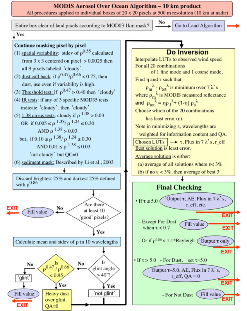
Figure 4: Flowchart of the over-ocean aerosol retrieval algorithm (adapted from Remer et al., 2005, updated for C6).     

4.6 Retrieved ocean products

As discussed earlier, the primary retrieved products of the ocean algorithm are the total τ at 0.55 μm (), the Fine (Mode) Weighting (η or η _0.55 )  and which Fine (f) and which Coarse (c) modes were used in the retrieval. The fitting error (ε) of the simulated spectral reflectance is also retrieved. Both the ‘best’ and ‘average’ solutions are reported. From these primary products a number of other parameters can be easily derived. Examples include the effective radius (r_eff) of the combined size distribution, the spectral total, fine and coarse t values (, and ), and a measure of the columnar aerosol mass concentration (M_C). Table 3 lists the products retrieved and derived during the ocean retrieval algorithm. Details about the ‘Quality_Assurance_Ocean’ (QA) SDS are given in the Appendix. Note that a parameter’s type does not indicate whether a parameter should be used in a quantitative way.  Each parameter must be independently validated via comparison with ground-truth measurements, where validation means that the product can be shown to be comparable with a set of ground-truth observations on a global scale, within some defined expected uncertainty. Prior to operational C6 processing, a testbed of 8 months of Aqua-MODIS granules were used to evaluate a few of the derived parameters. This provisional evaluation is described in Section 5. This ATBD document will be updated as the MODIS products are evaluated and reach validation status

  

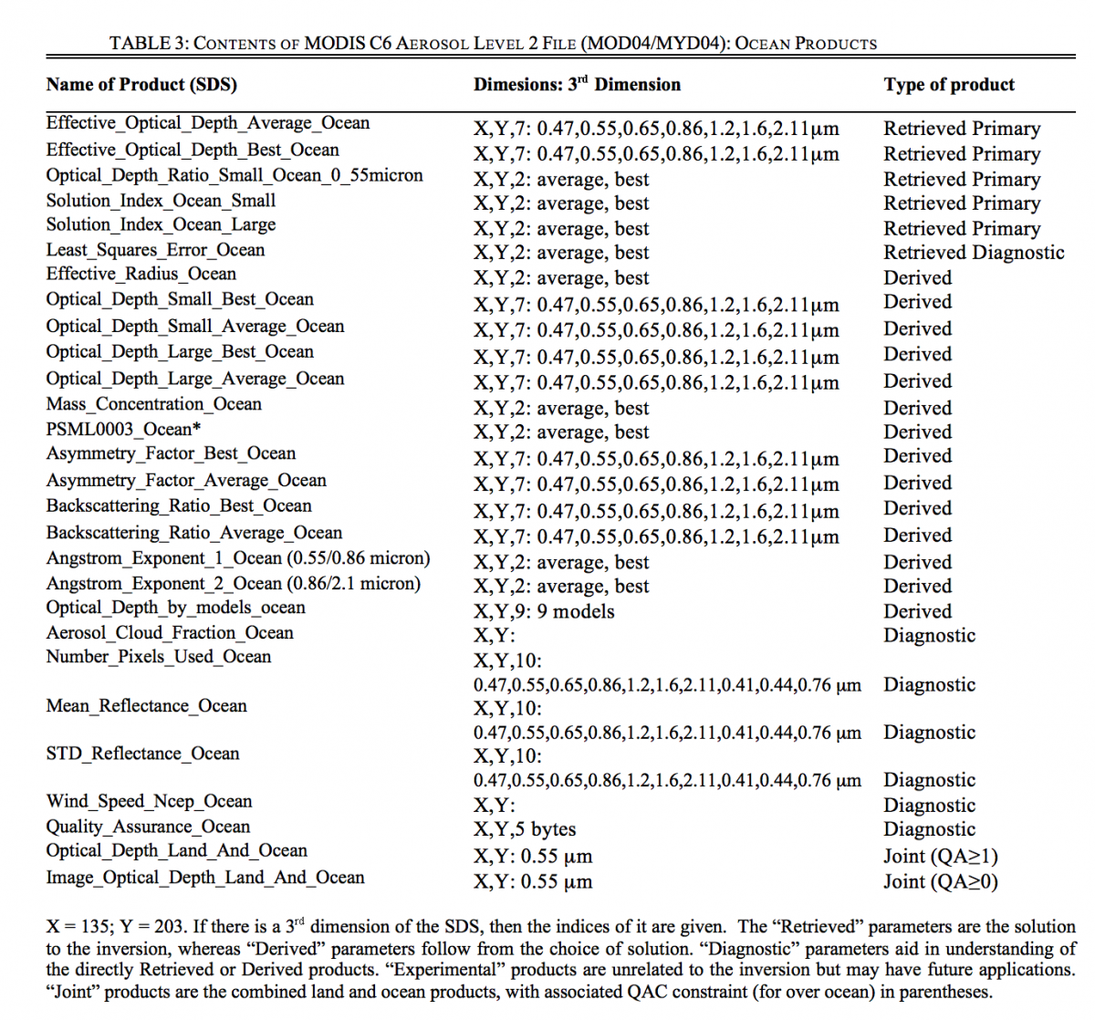
Some of the ocean products are combined with products from land (discussed in the next section) as the Joint products. For τ , two joint products are reported, the ‘Optical_Depth_Land_And_Ocean’ and the ‘Image_Optical_Depth_Land_And_Ocean’.  The first product is constrained by QAC whereas the “Image” product includes all QAC values in order to provide the most complete visulization of the AOD.