
A1: Gas corrections of L1B reflectance for aerosol retrievals in C6
The MODIS aerosol retrieval algorithm derives aerosol optical depth separately over land and ocean [Remer et al., 2005; Levy et al. 2007; 2009]. The retrieval algorithms use calibrated and geolocated L1B reflectances from MOD02 and MOD03 for Terra and MYD02 and MYD03 for Aqua MODIS products. Before the retrieval algorithm proceeds, the first step is to correct the L1B reflectance for atmospheric water vapor, ozone and dry gas. For this, appropriate ancillary data are acquired from National Center for Environmental Prediction (NCEP) analysis during the course of MODIS processing. These include the 1° X 1° global meteorological analysis data and 1° X 1° global Ozone data (created every six hours – format “gdas.PGrbF00.YYMMDD.HHz”). The primary parameters extracted from the NCEP data are total precipitable water vapor (PWAT or w in [cm]) and total column ozone O (in Dobson Units).In case the NCEP data are missing or invalid, the algorithm instead assumes fixed values of water vapor and ozone optical depths (US 1976 Standard Atmosphere climatological values).
For each L1B data pixel, the following gas transmission factors are calculated as a function of wavelength, air mass factor and some weighting coefficients, K. Table A1 lists the coefficients corresponding to each gas (water vapor, ozone and dry gas).
To calculate the air mass factor (G) we use the following approximation that is based on the assumption that the atmosphere is a simple spherical shell:
 (A1)
(A1)
If NCEP water vapor is valid, the transmission factor for water vapor is:
 (A2)
(A2)
If the NCEP water vapor is missing, then
 (A3)
(A3)
Ozone transmission is calculated in a similar way, that is:
 , (A4)
for a valid NCEP value, and
 , (A5)
when it is not.
TλDry Gas is the transmission factor due to dry gas, which includes CO2, CO, N2O, NO2, NO, CH4,O2, SO2, other trace gases and is given by:
 (A6)
(A6)
Therefore, The total gas transmission factor is a multiplication of all individual gas transmission terms, that is
 (A7)
(A7)
and the corrected reflectance is given by
 (A8)
(A8)
In Collection 6, we use 52 ECMWF profiles of H2O and O3 in the Line-by-line Radiative Transfer model (LBLRTM) to calculate the down welling water vapor and ozone transmittance in MODIS channels 1- 7 (see Table 1). The gas transmittance is weighted over the relative spectral response (RSR) of each of the 7 MODIS channels. These RSR weighted gas transmittance, gas content and air mass factors corresponding to 10 viewing zenith angles are used to calculate the gas correction coefficients for H2O and O3. This relationship between gas transmittance and columnar gas content is shown in Figure A1.1a and A1.1b for H2O and O3 respectively (i.e. Eq. A2 and Eq. A4).
The in the LBLRTM_v12.2 is used to calculate for H2O, O3 and Dry Gas in the 7 MODIS bands. In the absence of NCEP data, these H2O and O3 climatological optical depths are used to calculate their respective transmittance factors. For Dry Gas, however, the transmission factor is always calculated by using climatological optical depths.
The relative contribution of Rayleigh, water vapor, ozone and dry gas optical depths is shown in Figure A1.2.
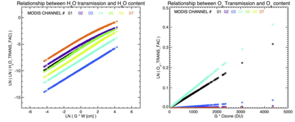
Figure A1.1: Relationship between Gas Transmission and Gas Content in the first 7 MODIS bands (a) H2O Transmission Factor vs. H2O content (cm) (b) O3 Transmission Factor vs. O3 content (DU)
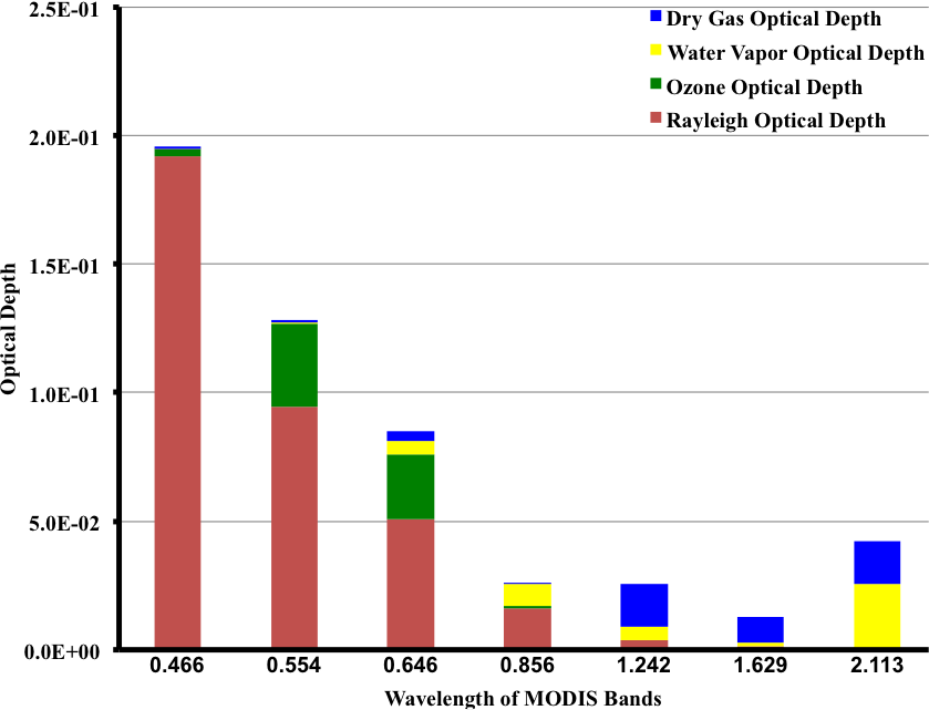
Figure A1.2: Relative contribution of Dry Gas, Water Vapor, Ozone and Rayleigh optical depths in the first 7 MODIS bands
A2: Masking over land and ocean
Masking clouds without masking aerosol events remains one of the most challenging issues faced by the aerosol retrieval algorithms. At Terra launch, the aerosol retrievals relied on the standard cloud mask products available in MxD35. Almost immediately we realized that these products were not going to be adequate. We learned that the 1.38 µm reflectance could be used to identify cirrus in the pixel. This channel is especially sensitive to cirrus clouds because in the absence of particles high in the atmosphere the channel returns reflectances near zero due to the strong water vapor absorption at this wavelength. A new cloud mask based on a spatial variability test, supplemented by cirrus tests using the 1.38 µm channel and a few remaining MxD35 products, was implemented in the over ocean aerosol algorithm (Martins et al., 2002). The mask proved to be very successful, especially after adjustments to the cirrus identification part of the algorithm (Gao et al. 2002). All of Collection 004 data over ocean, both from Terra and Aqua, were produced using this cloud mask.
A separate but similar cloud mask for masking clouds over land was developed later and not implemented until November 2002. The spatial variability cloud mask over land improved the aerosol retrievals, especially when it came to confusing heavy aerosol with cloud. However, isolated, residual cloud contamination in the product remained. In Collection 5, some adjustments to the technique were made.1.38 µm reflectance could either be slightly positive or slightly negative; The C4 aerosol algorithm required positive 1.38 µm reflectances while the C5 algorithm permitted negative reflectances, resulting in the recovery of many aerosol retrievals, especially over land. During C6 development, it became clear that the land cloudmasking algorithm was often masking dense smoke plumes as cloud, and that residual cloud contamination remained over ocean, particularly at cloud edges. Adjustments to the cloudmasking tests, described in sections A2.2 and A2.3, were made to the algorithm to address these two specific issues.
The following describes the steps for masking cloud and other unsatisfactory pixels when performing aerosol retrieval over land or ocean. Common to land and ocean are that the L1B reflectance data are corrected for gas absorption (Appendix 1) before masking tests are performed. If any of the pixels within the box are considered ‘land’ by the MxD35 cloud mask product, then the algorithm proceeds with the land retrieval algorithm. Only if all pixels in the box are ‘ocean’ is the ocean inversion performed. Separate cloud masks are used over land and ocean. Additional masks over land include snow and ice contamination as well as residual water bodies (such as lakes and swamps). The ocean retrievals require masking for glint and underwater sediments.
A2.1 Masking over ocean
Cloud Masking Over Ocean
If all 400 pixels in the 10km box are considered to be ‘water’ then the ocean algorithm is followed. After the gas correction described in section A1.1, the algorithm has the arduous task of separating 'good' pixels from 'cloudy' pixels. The standard MxD35 cloud mask includes using the brightness in the visible channels to identify clouds. This procedure will mistake heavy aerosol as 'cloudy', and miss retrieving important aerosol events over ocean. On the other hand, relying on IR-tests alone permits low altitude, warm clouds to escape and be misidentified as 'clear', introducing cloud contamination in the aerosol products. Thus, our cloud mask over ocean combines spatial variability tests (e.g. Martins et al., 2002) along with tests of brightness in visible and infrared channels.
The algorithm marches through the 10 by 10 box, examining the standard deviation of ρ0.55 in every group of 3 by 3 pixels. If the group of 9 pixels has a standard greater than 0.0025, then the center pixel is labeled as 'cloudy', and is discarded (Martins, et al. 2002). The only exception to this rule is for heavy dust, which may at times be as spatially inhomogeneous as clouds. Heavy dust is identified by its absorption at 0.47 µm using the ratio (ρ0.47/ρ0.65). This quantifies the difference that our eyes witness naturally. Dust absorbs at blue wavelengths and appears brown. Clouds are spectrally moderately absorbing and appear white to our eyes. If ρ0.47/ ρ0.65 < 0.75, then the central pixel of the group of 9 is identified as 'dust' and will be included in the retrieval even if it is inhomogeneous. This is a conservative threshold that requires very heavy dust in order to avoid clouds. Less restrictive thresholds would permit more dust retrievals, but might accidentally permit cloud contamination.
The spatial variability test separates aerosol from most cloud types, but sometimes fails at the centers of large, thick clouds and also with cirrus, both of which can be spatially smooth. The centers of large, thick clouds are very bright in the visible, and so we identify these clouds when r0.47> 0.40. This is an extremely high threshold that translates into an aerosol optical thickness greater than 5.0, but only for non-absorbing aerosol. Absorbing aerosol never reaches that high value of reflectance and will pass this cloud test unscathed. Some high values of non-absorbing aerosol may be discarded along with bright clouds, but this confusion is rare. Most heavy aerosol loading, with τ > 5.0, absorbs somewhat at 0.47 µm and fails to reach the 0.40 threshold value, exhibited by very bright white clouds.
Cirrus clouds are identified with a combination of infrared and near-infrared tests. Three infrared tests provided by the standard MODIS cloud mask, MxD35, are examined. The three IR tests are the “Thin Cirrus (IR) Test” (Bit 11), the “High Cloud (6.7 μm) Test” (Bit 15), and the “IR Temperature Difference Test” (Bit 18). If any of these three tests register as “applied”, then the 2×2 box of 500 m pixels (1 km MxD35 pixel) is denoted as “cloudy”, and none of these pixels are retained for aerosol retrieval. The near-infrared cirrus test is based on the reflectance in the 1.38 µm channel and the ratio r1.38 / r1.24 (Gao, et al. 2002). It is applied in the algorithm as a three step process. If ρ1.38 / ρ1.24 > 0.3, then the pixel is 'cloudy'. If 0.005 ≤ r1.38 / ρ1.24 ≤ 0.30 and ρ1.38 > 0.03 and ρ0.65 > 1.5ρray.0.65, then the pixels is also 'cloudy'. However, if 0.005 ≤ ρ1.38 / ρ1.24 ≤ 0.30 and 0.01 ≤ ρ1.38 ≤ 0.03 and ρ0.65 > 1.5ρray.0.65, then the situation is ambiguous. The algorithm labels the pixel as 'not cloudy' and will include the pixel in the retrieval process, but the quality of the retrieval (Quality Assurance Confidence - QAC) is reduced to 0, 'poor quality'. This permits aerosol retrieval at the orbital level (Level 2), but prohibits the retrieval from contributing to the long-term global aerosol statistics (Level 3). Only retrievals with QAC > 0, contribute to the Level 3 Quality Weighted products. The products and product levels are explained further in Section 3. If the reflectance at 0.65 µm (ρ0.65) does not exceed 1.5 times the Rayleigh reflectance in that channel (ρray.0.65) or the reflectance at 1.38 µm does not exceed 0.01, then the pixel is assumed to be 'not cloudy' with no ambiguity, unless the ratio ρ1.38 / ρ1.24) exceeds 0.3.
In the transition from C5 to C6, the MOD35 team identified that the IR Temperature Difference Test was falsely identifying clear ocean as cloudy in the tropics. The test was relaxed to increase clear ocean retrievals, but in testing, the aerosol team found that the MOD35 cloud mask change also increased cirrus contamination. Therefore, we lowered the ρ1.38 / ρ1.24 reflectance ratio threshold from 0.10 to 0.005 to initiate the testing for cirrus contamination. An example granule showing reduced cloud contamination in C6 as compared to C5 over ocean is shown in Figure A2.1.
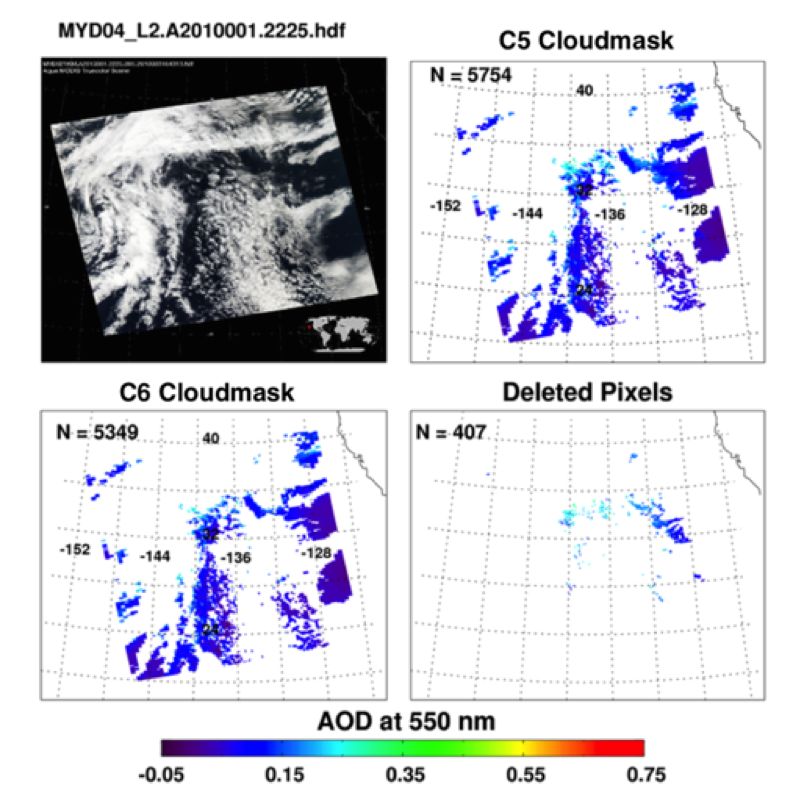
Figure A2.1, Granule retrieved over the Pacific Ocean from MODIS- Aqua taken on 1 January 2010 at 22:25UTC. Top left: true color (RGB) showing scene taken from modis-atmos.gsfc.nasa.gov. (b and c) Retrieved high quality (QAC≥1 over ocean) AOD at 0.55 μm, without/with the revised 1.38 μm cloud mask test. (d) Cirrus contaminated pixels that have been removed over ocean. From Levy et al., 2013.
Ocean sediment mask
The final mask applied to the data is the sediment mask, which identifies which ocean scenes are contaminated by river sediments (Li et al, 2002) and discards those pixels. The sediment mask takes advantage of the strong absorption by water at wavelengths longer than 1 µm. The resulting spectral reflectances over water with suspended sediments thus show elevated values in the visible, but not in the longer wavelengths. This creates a unique spectral signature quite different from clear ocean water and also different from airborne dust.
A2.2 Masking over land
Cloud Masking Over Land
The algorithm generates a cloud mask over land using the mean weighted spatial variability of the 0.47 µm (>0.0025) and 1.38 µm (> 0.003) channel reflectance, as well as the absolute value of the 0.47 µm reflectance (>0.4) and the 1.38 µm reflectance (> 0.025). The combination of the two channels yields information about both visibly bright thick clouds and visibly dim thin cirrus. Note, that the refl_1.38 < 0.025 threshold allows cirrus contamination into the land aerosol retrieval. However, those retrievals will have QAC (Quality Assurance Confidence) set to zero.
The visible channel reflectance spatial variability test for land is similar to that for ocean (as described by Martins et al., (2002)), although the 0.47 µm channel (at 500 m resolution) is used instead, and the algorithm calculates the mean weighted standard deviation (Equation 1) of the reflectance of each group of 3 x 3 pixels. If that standard deviation is greater than 0.0025, then the center pixel of the 3x3 pixel box is considered a cloud. During C6 development, both Witte et al. (2011) and van Donkelaar et al. (2011) noted that operational MODIS aerosol retrieval failed to capture the extreme Russian fire events of 2010. Retrieval of the extremely heavy smoke (AOD ≫ 1.0) in the middle of the plumes required either turning off the cloud mask, or finding a suitable aerosol “call-back” test. Because dense smoke plumes tend to be both more spatially variable and brighter than more widespread aerosol hazes, the mean weighted spatial variability test was too conservative. To help retrieve some of these smoke pixels, the cloud mask over land was modified for C6. For pixels that fail the mean weighted spatial variability test, an additional test is applied. If the straight (not mean weighted) standard deviation of the 3x3 pixel box is less than 0.0075, the pixel is considered to be clear even if it failed the mean weighted spatial standard deviation test. An example of the change is shown in Figure A2.2. It is noteworthy that the change to the cloudmask test still does not retrieve the entire smoke plume, more details of the limitations of aerosol cloudmasking in heavy smoke is provided in Livingston et al., 2013.
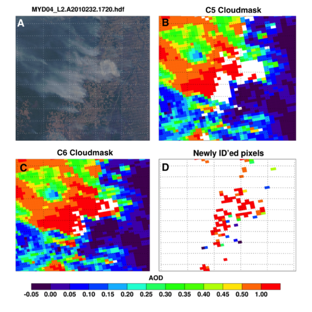
Figure A2.2, Granule retrieved over Brazil from MODIS-Aqua observed on 20 August 2010 at 17:2- UTC. Top left: true color (RGB) showing intense smoke plumes. (b and c) Retrieved high quality (QAC≥=3 over land) AOD at 0.55 μm, without/with the revised spatial variability test. (d) Smoke plume pixels that have been successfully retrieved with the C6 cloudmask that were masked in C5.
The visible channel reflectance threshold test is also performed on the 0.47 µm channel. These are performed pixel by pixel (500 m resolution). If the reflectance at 0.47 µm is greater than 0.4, the pixel is considered a cloud, and all channels are cloud masked for the 500 m pixel.
The 1.38 µm channel reflectance spatial variability and threshold tests are analogous to those in the visible, however, as the resolution is 1 km, the tests cover a larger area. If the spatial variability test finds that the 3x3 pixel standard deviation is greater than 0.003, then the center pixel is cloud masked for all channels. Pixels with a 1.38 µm reflectance greater than 0.025 are considered cloud, and pixels with a 1.38 µm reflectance greater than 0.01 and less than 0.025 are considered cloud free and retrievable, but the resulting AOD retrieval will be assigned a QAC value of 0 .
The final cloud mask is the union of the four cloud mask tests described above.
Snow and inland water masking
A number of other tests are performed at a variety of resolutions to remove contamination by “wet” pixels, including snow fields, swamps, and inland water bodies. These pixels would be expected to have poorly behaved VISvs2.11 surface reflectance relationships. Note that the reflectance data have already been cloud masked and corrected for gas absorption.
The snow/ice mask determined by an NDVI-like ratio of 0.86 µm and 1.24 µm channel reflectances (at 500 m resolution), i.e.  , and the brightness temperature of the 11 µm MODIS thermal band (channel 31 – interpolated to 500 m resolution). If the ratio is greater than 0.1 and the 11 µm brightness temperature is less than 285K, then the pixel is considered a snow or ice contaminated and masked [Li et al., 2005]. Figure A2.3 shows an example of improvements gained by the snow mask.
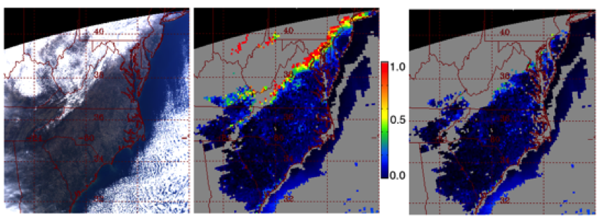
Fig. A2.3. (a) – An Aqua MODIS image over North America on February 8, 2004; (b) the derived aerosol optical depth image using the Collection 004 MODIS aerosol algorithm; and (c) the Collection 005 aerosol optical depth image with improved snow masking.
The inland water mask is determined by computing the traditional NDVI for the 0.65 µm and the 0.86 µm channels 250 m resolution, i.e.  . If the NDVI value is greater than 0.1 it is considered an inland water body.
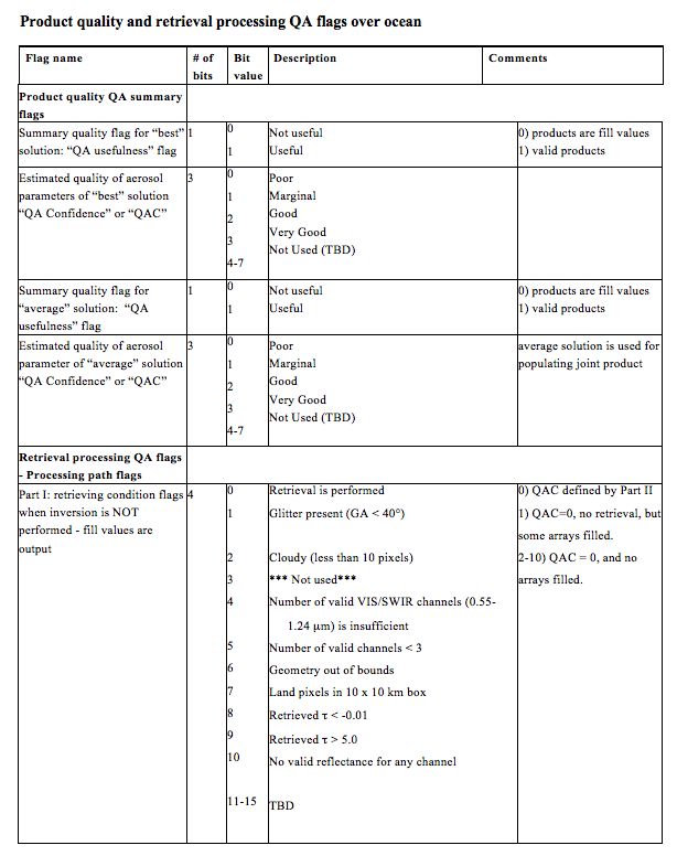
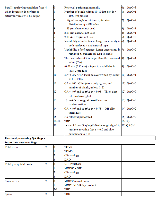
A3: Table of run time QA flags of MxD04 level 2 aerosol products
This appendix updates the information for dark target aerosol flags, given in the QA plan for C6 (MODIS Atmosphere QA Plan for Collection 6) available online at (http://modis-atmos.gsfc.nasa.gov/reference_atbd.html).
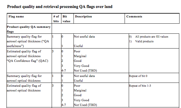
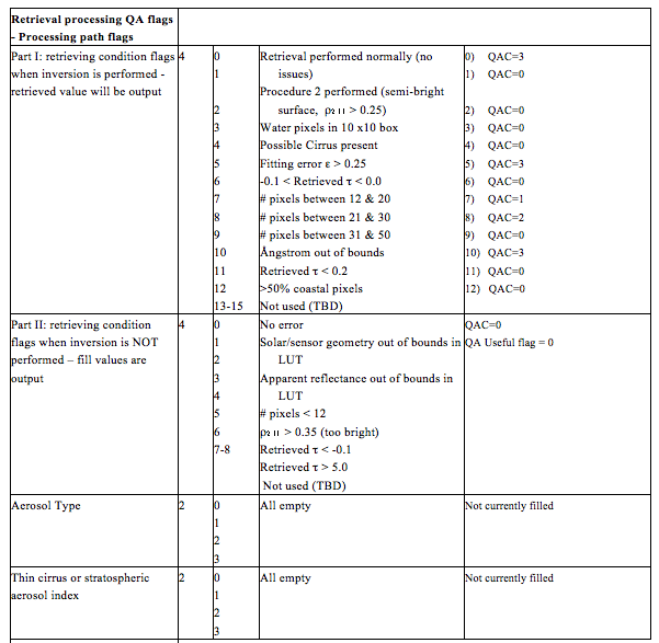
The aerosol (dark target) run time Quality Assurance (QA) flags are stored as three Scientific Data Sets (SDSs); Quality_Assurance_Land, Quality_Assurance_Ocean, and Land_Ocean_Quality_Flag. The ‘Land_Ocean_Quality_Flag’ SDS is an integer between 0 and 3 that provides the quality assurance confidence (QAC) of the retrieval pixel, where 0=bad, 1=marginal, 2=good and 3=very good. The two other SDSs are five bytes that provide information on the processing (logic) path taken during the aerosol retrieval. The aerosol QA includes product quality flags, retrieval processing flags, and input data resource flags which are designed separately for land and ocean because of the differences of retrieval algorithms. Particular flags may indicate: a) conditions why retrieval was not attempted at all (e.g. input data outside of boundary conditions), b) cases where input data quality may be poor (e.g. large cloud fraction), so that the retrieval is performed with lower confidence, or c) cases where retrieval may have been performed but the results were poor (e.g. results outside of realistic physical conditions).
The Quality Assurance confidence (QAC) flag given in the ‘Land_Ocean_Quality_Flag’ SDS summarizes the QA logic, and are referred to in the main text of this ATBD. These flags are also given within the ‘Quality_Assurance_Land’ and ‘Quality Assurance_Ocean’ SDSs. The QAC flags are the ‘Estimated quality flag of aerosol optical thickness at 0.47 µm’ land retrievals and the ‘Estimated quality of aerosol parameter of average solution’ for ocean retrievals.
All Aerosol QA Flag arrays have the following characteristics:
• Spatial resolution: 10 x 10 km for MxD04_L2, 3 x 3 km for MxD04_3K
• Processing mode: Day time mode only
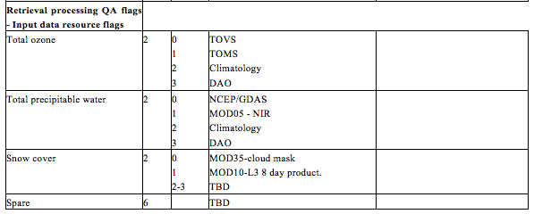
The following tables describe the byte decoding of the MxD04 Quality_Assurance_Land, and Quality_Assurance_Ocean SDSs. Each flag corresponds to a certain number of bits, and bit values corresponding to results of certain tests. Note that the flags representing the case of valid retrieval but lower confidence is known as “Part I” over land, but “Part II” over ocean. Similarly the flags representing the case of no valid retrieval are known as Part II over land, but Part I over ocean. Under the column “Comments”, we list how other flags may be reset (if applicable). For example, if Part I over land receives the value of 8 (less than optimal clear sky pixels) then the QAC bits will be set to 2 (good quality).
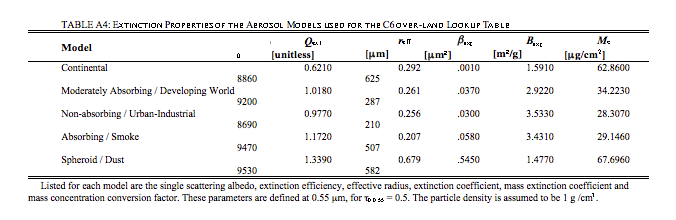
A4: Calculation of mass concentration
The following equations lead to derivation of Mass Concentration in units of [mg per cm2]. In these equations: dN/dlnr is the number size distribution with r denoting radius (in µm). For a lognormal mode, rg is the geometric mean radius, s is lnsg representing the standard deviation of the radius, and N0 is the number of particles per cross section of the atmospheric column (i.e. the amplitude of the lognormal size distribution). In our case, we assume that the distribution is normalized, so that N0=1.
The number N is related to the volume V and area A distributions by:
 (A9)
(A9)
N0, V0, and A0 are the amplitudes of the corresponding distributions, i.e.
 (A10)
(A10)
For a single lognormal mode defined by:
 (A11)
(A11)
the Moments of order k, Mk are defined as
 (A12)
(A12)
The effective radius reff in [µm] is defined by the moments, i.e.
 (A13)
(A13)
The extinction coefficient, Βext is related to the extinction efficiency Qext through the area distribution, and is specific to each mode
 (A14)
(A14)
These parameters are calculated via Mie code (MIEV, [Wiscombe, 1980]). Note that the scattering coefficient Βsca and efficiency Qsca are related the same way. The mass extinction coefficient Bext is in units of [area per mass] and depends on the extinction efficiency and the particle density r (assumed to be 1 g per cm3), such that
 (A15)
(A15)
(Chin et al., 2002). For a single lognormal mode,
 (A16)
(A16)
However our aerosol models are sums of multiple modes, so that the area and volume distributions must take into account the contributions of each mode. If there are two modes, (i.e. modes 1 and 2), reff must be calculated this way:
 (A17)
(A17)
Similar modifications are made when calculating Q and thus B.
We can define the Mass Concentration conversion factor, Mc, as the inverse of B, such that
 (A18)
(A18)
The columnar mass concentration, M [mass per area] is then defined as
 (A19)
(A19)
The final columnar mass concentration product is a weighted combination of the fine and coarse model ts (τ f and τ c) and the mass concentration coefficients of each model, i.e.,
 (A20)
(A20)
A5: Merged Deep Blue / Dark Target SDSs
The dark target algorithm over land (e.g., Levy et al., 2007a and b) is not designed to retrieve aerosol over bright surfaces, including desert. This leaves significant holes in global aerosol sampling. However, in recent years, Hsu et al. (2004, 2006) have developed an algorithm that retrieves aerosol properties over brighter surfaces. This algorithm, known as Deep Blue (DB), makes use of the observation that even visually bright desert scenes are have low surface reflectance and are relatively stable in the deep-blue wavelengths (e.g., 0.41 and 0.47 μm). The DB algorithms have also been revised for C6, and notably will now also provide coverage over vegetated land surfaces (Sayer et al., 2013; Hsu et al., 2013); therefore, there are land areas that can be retrieved by both DB and DT algorithms.
For C6, we introduce a new “best-of ” AOD product that combines DB, DT-land and DT-ocean. This will be reported by the SDS named “Dark_Target_Deep_Blue_Optical_Depth_550_Combined”. A climatology from the MODIS-derived, monthly, gridded NDVI product (MYD13C2, Huete et al., 2011) is used as a map for assigning which algorithm takes precedence. This database is a set of 12 multiannual monthly means, gap-filled using the nearest month. If (NDVI > 0.3) then use the results from DT (τ_DT). If (NDVI < 0.2) then use results from DB (τ_DB). For the transition areas (0.2 ≤ NDVI ≤ 0.3), the routine considers the confidence as indicated by QAC values (Q_DT and Q_DB), where high confidence means Q_DT = 3 or Q_DB ≥ 2. If both are high confidence, the AOD is the average of the two, in other words,
τ =(τ_DT+τ_DB)/2.
If only one retrieval has high confidence, then the AOD is assigned to that retrieval. If neither has high confidence, then the combined AOD remains undefined.
Table A5 reports the new SDSs referring to the DT/DB merging. Figure A5 shows this combined product (DBDT) for the four months of 2008, and compares it with the original DT product. DBDT increases coverage over both dark and bright surfaces (except snow and clouds), and in certain geographical regions, such as Australia and southwestern Asia, DBDT not only increases coverage but also modifies the AOD. A comprehensive analysis of the differences in retrieved AOD from DT, DB and the DBDT merged product is provided in Sayer et al., 2014.
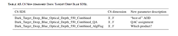
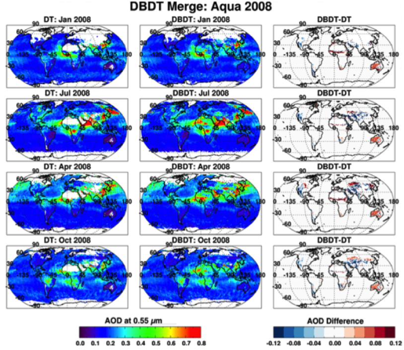
Figure A5: Global map of Aqua-derived AOD (at 0.55 μm) for four months (January, April, July and October) in 2008. Plotted for each month Oct) in 2008. Plotted for each month are: DT only (left), merged DT/DB (center), and differences between DBDT and DT, for grids where DT retrieves (right).
A6: New cloud diagnostic products
For C6, there will be a new array of cloud diagnostics reported in the MxD04 file, including two products offered at 500 m resolution (Table A6). During the cloud masking operations (separate for land and ocean), the algorithm keeps track of whether a given 500m pixel is considered to be “cloudy” or “clear”. This information is carried along in an array of bits (0 = cloudy, 1 = clear) and reported as “Aerosol_Cldmsk_Land_Ocean”. As this cloud mask is created, the algorithm also determines the distance from every pixel to the nearest “cloudy” pixel. This is “Cloud_Distance_Land_Ocean”. The intention is that users concerned about aerosol retrievals affected by cloud adjacency effects (3-D effects) or by humidified aerosols and cloud fragments in cloud fields (twilight zone) can trace exactly which pixels were used in the retrieval or plot the retrievals as a function to the nearest cloud. There is also a 10 km product that offers the average distance to the nearest cloud of all the pixels within the 10 km box used by the retrieval, i.e., “Average_Cloud_Distance_Land_Ocean”. An example of the 500 m parameters is shown in Figure A6.
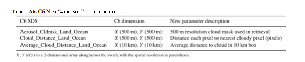
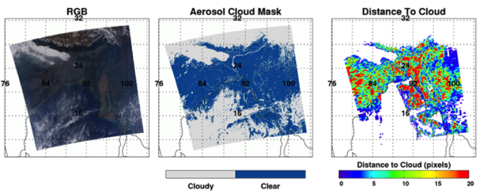
Figure A6: New aerosol cloud mask variables, both from an Aqua granule on 3 January 2010 at 07:20 UTC. (a) RGB, (b) Aerosol cloud mask, (c) Distance to cloud (in pixels).