5. Algorithm description: land
Theoretical background
The upward reflectance (normalized solar radiance), at the top of the atmosphere (TOA), is a function of successive orders of radiation interactions, within the coupled surface-atmosphere system. The TOA angular (θ0, θ and Φ = solar zenith, view zenith and relative azimuth angles) spectral reflectance (ρλ(θ0, θ, Φ) ) at a wavelength results from: scattering of radiation within the atmosphere without interaction with the surface (known as the ‘atmospheric path reflectance’), the reflection of radiation off the surface that is directly transmitted to the TOA (the ‘surface function’), and the reflection of radiation from outside the sensor’s field of view (the ‘environment function’). The environment function is neglected so that to a good approximation:
 (28)
(28)
where ρaλ is the atmospheric ‘path reflectance’, Tλ(θ0) and Tλ(θ) is the downward and upward atmospheric transmissions (reciprocity implied), sλ is the atmospheric backscattering ratios, and ρsλ is the angular spectral surface reflectance.
Except for the surface reflectance, each term on the right hand side of Equation 28 is a function of the aerosol type and loading (τ). Assuming that a small set of aerosol types and loadings can describe the range of global aerosol, we can derive a lookup table that contains pre-computed simulations of these aerosol conditions.The goal of the algorithm is to use the lookup table to determine the conditions that best mimic the MODIS-observed spectral reflectance ρmλ, and retrieve the associated aerosol properties (including τ and η). The difficulty lies in making the most appropriate assumptions about both the surface and atmospheric contributions.
5.1 Strategy
The C6 Land (C6-L) algorithm is a minor update from C5-L, which in turn was a complete overhaul from C4-L (Levy et al., 2007a,b). The C5-L/C6-L algorithms retrieve aerosol properties in three channels simultaneously (the two visible channels, plus the 2.11 μm channel) and assume that the 2.11 μm channel contains information about coarse mode aerosol as well as the surface reflectance. The surface reflectance in the visible can be determined as a function of the surface reflectance at 2.11 μm, as well as a function of the scattering angle and the “greenness” of the surface in the mid-IR spectrum (NDVI-like parameter based on 1.24 and 2.11 μm reflectance).
Like the ocean algorithm (C6-O), the C6-L algorithm is an inversion, but takes only three (nearly) independent observations of spectral reflectance (0.47, 0.65 and 2.1 μm) to retrieve three (nearly) independent pieces of information. These include total t at 0.55 μm (τ0.55), Fine (model) Weighting at 0.55 μm (η or η0.55 ), and the surface reflectance at 2.1 μm (ρ s2.12). Like the ocean algorithm, C6-L is based on look-up table (LUT) approach, i.e., radiative transfer calculations are pre-computed for a set of aerosol and surface parameters and compared with the observed radiation field. The algorithm assumes that one fine-dominated aerosol model and one coarse-dominated aerosol model (each may be comprised of multiple lognormal modes) can be combined with proper weightings to represent the ambient aerosol properties over the target. Spectral reflectance from the LUT is compared with MODIS-measured spectral reflectance to find the best match. This best fit is the solution to the inversion.
5.2 Formulation of the land algorithm
Because the C6-L algorithm is only a modest update, we describe the formulation of the C5-L algorithm while noting specific changes that have been made for C6-L. In order to construct the aerosol models for use in C5-L (see section 4.3), we generated a large data set of AERONET L2A (quality assured Level 2 data) sunphotometer (http://aeronet.gsfc.nasa.gov) data co-located with the MODIS C4 (Ichoku et al. 2002) observations. From the AERONET database, we used a combination of direct ‘sun’ measurements of t in four or more wavelengths (at least 0.44, 0.67, 0.87 and 1.02 μm) and indirect ‘sky’ measurements of almucantur radiance that were inverted into aerosol optical properties and size distributions. Sun measurements are made approximately every 15 minutes, whereas almucantur sky measurements are performed about every hour. Fine aerosol Weighting (η) is also estimated from an inversion of the sun-measured spectral τ(O’Neill et al., (2003). Over 15,000 pairs of MODIS and AERONET sun data, at over 200 global sites, were co-located in time via the technique of Ichoku et al., (2002). A valid MODIS/AERONET match is considered when there at least five (out of a possible 25) MODIS retrievals (10 km x 10 km resolution) within the box, and at least two (out of a possible five) AERONET observations within an hour. About 136,000 individual AERONET sky retrievals were used to develop the C5-L global/seasonal aerosol climatology.
5.3 Aerosol optical models and lookup tables
A number of studies (e.g. Chu et al., 2002, Remer et al., 2005, Ichoku et al., 2002, Levy et al., 2005) have demonstrated that C4-L MODIS/AERONET regression of τ over land resulted in slope less than one; meaning that MODIS tended to under-retrieve optical depth for large τ. This indicated that the aerosol models used in C4-L were not truly representative of the optical conditions viewed by MODIS. For example, over the east coast of the United States during summertime, Levy et al. (2005) showed MODIS retrievals would be improved by switching to the GSFC urban/industrial aerosol model derived from AERONET data (Dubovik et al., 2002). Omar et al., (2005) performed a “cluster analysis” of AERONET data and found that six aerosol models (composed of desert dust, biomass burning, background/rural polluted continental, marine, and dirty pollution, respectively) sufficiently represented the entire AERONET dataset. The models varied mainly by their aerosol scattering and absorption qualities expressed as w0 and size distribution (asymmetry parameter, g). Two models were representative of very clean conditions (marine and background/rural). One of the models (dust) was coarse-dominated, analogous to the MODIS coarse dust model, and three were fine models having different ω0 (biomass burning, polluted continental, and dirty pollution), that were analogous to the C4-L set of fine models. Because the MODIS over-land retrieval employs only three channels (and suffers from surface and other contaminations), there is not enough information available for the algorithm to select a fine aerosol model. Therefore, the aerosol retrieval algorithm must assign the fine aerosol model a priori of the retrieval. This section describes how cluster analysis was used to determine a set of global aerosol models, and how they were assigned as a function of location and season. More information is in Levy et al., (2007a) and Levy et al., (2013). Note that the “continental model” mentioned throughout this document and described in table 4 is only used for “Procedure B: Alternative Retreival for Brighter Surfaces” decribed below in section 5.5.
For the C5-L cluster analysis, we used all AERONET Level 2 (L2A) data that were processed as of February 2005, encompassing both spherical and spheroid retrievals. We filtered the retrievals in accordance with the minimum quality parameters suggested by the AERONET team, including: τ at 0.44 μm greater than 0.4, solar zenith angle greater than 45°, 21 symmetric left/right azimuth angles, and radiance retrieval error less than 4%. The resulting data set was comprised of 13,496 spherical retrievals and 5128 spheroid retrievals at over 100 sites. We separated the AERONET data set into ten discrete bins of τ and used each one separately to differentiate aerosol types. Presumably, this would help to identify expected dynamic properties (function of τ) of each aerosol type (e.g. Remer et al., (1998)). In contrast to Omar et al. (2005), we desired to pursue not necessarily the most statistically significant clustering, but rather to identify three distinct fine-dominated models useful for MODIS. With this goal of fine model identification in mind, we clustered with respect to only two optical parameters: ω0 at 0.67 μm and the asymmetry parameter g at 0.44 μm. We used ω0 as the criteria to distinguish between non-absorbing aerosols (such as urban/industrial pollution – (Remer et al., 1998; Dubovik et al., 2002)) and much more absorbing aerosols (such as savanna burning smoke – (Ichoku et al., 2003; Dubovik et al., 2002)), and g at 0.44 μm to differentiate between relative size (via the phase function) of primarily fine aerosols. We numbered the clusters so that in each τ bin, there is always a ‘low’, ‘medium’ and ‘high’ cluster, and upon re-combination across τ bins, that they would yield dynamical information. As for the coarse aerosol model, we found that a single cluster described the spheroid-based almucantur inversions (Dubovik et al., 2006). Since the sites contributing to spheroid data were primarily those known to be in dust regions, we assumed that the spheroid model represented coarse (‘dust’) aerosol.
Since the development of the C5-L aerosol models in 2007, there have been thousands of size distribution retrievals at the same and additional AERONET sites around the globe. In addition, there have been many updates to the AERONET retrieval itself (http://aeronet.gsfc.nasa.gov) including updates of non-spherical dust assumptions and retrieval of non-spherical fraction (Dubovik et al., 2006). Instead of using the same surface reflectance assumptions for all almucantar inversions, the newer AERONET Version 2 inversion products use surface spectral albedo climatology as determined by MODIS (Holben et al., 2006). According to studies of the version 2 AERONET products, retrieved size distributions, refractive indices and single scattering albedos, at least at some sites, have changed significantly from those reported for Version 1 (Giles et al., 2012). Since there have been changes to AERONET climatology, we investigated whether the C6-L MODIS aerosol model assumptions, based on this climatology, would require an update.
Using the same methodology as described by Levy et al. (2007a), we performed a cluster analysis of the entire AERONET climatology through 2010. Surprisingly, while a few sites showed significant differences from that observed by the prior analysis, the overall pattern was unchanged. In general, the global aerosol type could be separated into fine-mode dominated (fine models) and coarse-mode dominated (coarse models), with the fine models further separated into being strongly absorbing, moderately absorbing and weakly absorbing. Although there were slight changes for each fine model’s optical properties, they were not significant enough to justify revision. Thus, for C6-L, the models are unchanged from C5-L.
For each AERONET site, and for each season, we filtered for only spherical aerosol type, and then determined the percentage of the non-dust retrievals attributed to each cluster. Figure 5 (a-d) displays pie-plots at each site, as a function of season. To remove poor statistics, we show pie plots only at sites having at least 10 observations (per season) throughout the history of AERONET. Green pie segments represent the non-absorbing (ω0~0.95) model (presumably urban/industrial aerosol), blue segments are the moderately absorbing (ω0~0.90) model (presumably background, forest smoke and developing world aerosol), and red segments designate the highly absorbing (ω0~0.85) model (presumably savanna/grassland smoke aerosol). At most sites and most seasons, the aerosol type is as expected. Non-absorbing aerosol (green) dominates the U.S. East Coast and far western Europe, whereas highly absorbing aerosol (red) dominates the savannas of South America and Africa. Most other sites are dominated by moderately absorbing aerosol (blue) or are a mix of all clusters. There are some exceptions to expectation, however. Southeast Asia seems to be primarily non-absorbing aerosols in JJA and SON, and is absorbing during DJF, as opposed to the absorbing aerosol assumed in C4-L. Studies (e.g. Eck et al., 2005) confirm that the urbanized areas of Southeast Asia are primarily non-absorbing.
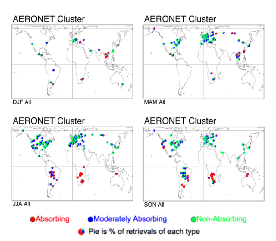
Figure 5: Percentage (pie charts) of spherical aerosol model type retrieved at each AERONET site per season. Colors represent absorbing (ω0 ~ 0.85), moderately absorbing (ω0 ~ 0.90) and non-absorbing (ω0 ~ 0.95), respectively.
Keeping in mind our goal of dividing the world into plausible aerosol types, we decided that each site should have an assumed aerosol type attached to it. The moderately absorbing aerosol model was set as the default, and would be overridden only if clear dominance of one of the other two aerosol types was observed. If either the non-absorbing or the absorbing aerosol occupied more than 40% of the pie, and the other occupied less than 20%, then the site was designated as the dominant aerosol type. For example, GSFC (Longitude = -77; Latitude = 37.93) during the summer months (JJA) recorded 87% non-absorbing and 13% moderately absorbing, meaning it would be designated as non-absorbing. Figure 6 (a-d) displays the designated aerosol types at each site. As in Figure 5, green represents non-absorbing, blue represents moderately absorbing and red designates absorbing aerosol types. Most site designations seem reasonable and were expected from our experience. North America during the summer (JJA) is split between non-absorbing and moderately absorbing aerosol types, much the same way (approximately -100° longitude) as was prescribed for C5. Southern Africa during the winter season (DJF) is solidly designated as absorbing aerosol (e.g. Ichoku et al., 2003). Western Europe is evenly split between non-absorbing and moderately absorbing, meaning that a subjective decision is needed here. The non-absorbing aerosol model was chosen for Western Europe.
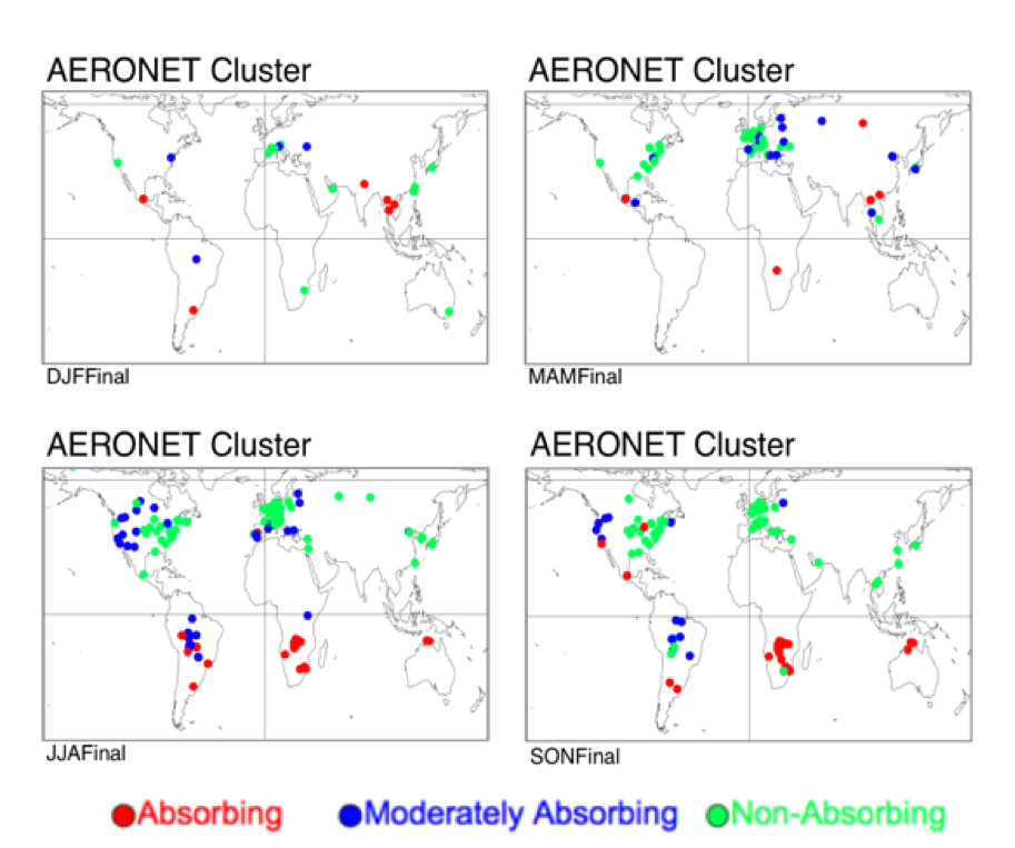
Figure 6: Final spherical aerosol model type designated at each AERONET site per season. Colors represent absorbing (ω0 ~ 0.85), moderately absorbing (ω0 ~ 0.90) and non-absorbing (ω0 ~ 0.95), respectively.
Figure 7 plots the final decision for designating aerosol types around the globe, as a function of season. Note that where possible the shapes correspond with the clustering. At some regions, however, some subjectivity was needed to connect areas. For example, even though insufficient data exists for Africa north of the equator, the known surface types and seasonal cycles suggest that heavy absorbing aerosol would be produced during the biomass burning season. Red designates regions where the absorbing aerosol is chosen, whereas green represents non-absorbing aerosol. The moderately absorbing (ω0 ~ 0.90) model is assumed everywhere else. These images were mapped onto a 1° longitude x 1° latitude grid, such that a fine aerosol type is assumed for each grid point, globally. This global map approach, that is not hardwired into the processing code, will allow for easy alterations as new information becomes available. While the overall spatial distribution of aerosol types remained the same as defined for C5, there was much larger AERONET sampling, and more opportunity to fine-tune the model distribution borders. The obvious change from C5 is that the border contours are now drawn by hand, to account for mountainous terrain that separate aerosol regimes. Differences are seen over the Amazon (aerosol is now assumed moderately absorbing, consistent with Schafer et al., 2008), over southeastern Asia (now more absorbing), and over the western United States (now clearly separated by the Rocky mountains).
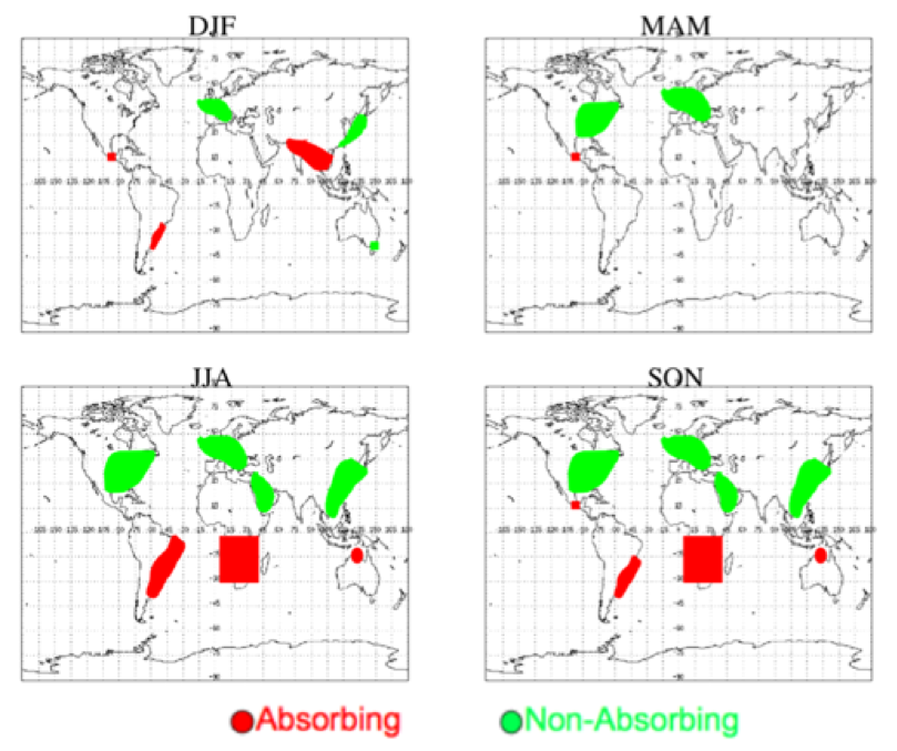
Figure 7: Final spherical aerosol model type designated at 1° x 1° gridbox per season. Red and green represent strongly-absorbing (ω0 ~ 0.85) or weakly-absorbing (ω0 ~ 0.95) models, respectively. Moderately absorbing (ω0 ~ 0.90) is assumed everywhere else.
Table 4 displays the optical properties and size distributions for the three spherical (moderately absorbing, absorbing and non-absorbing) fine-dominated models and the one spheroid coarse aerosol (dust) model, and the Continental model. Figure 8 shows the size distributions for the four AERONET-derived models. Note the dynamic nature (function of τ) of the size properties of the fine models, especially the non-absorbing model. Figure 9 plots the final phase function at 0.55 μm for each model as well as spectral dependence of three parameters (τ, ω0 and g), all for τ0.55 = 0.5.
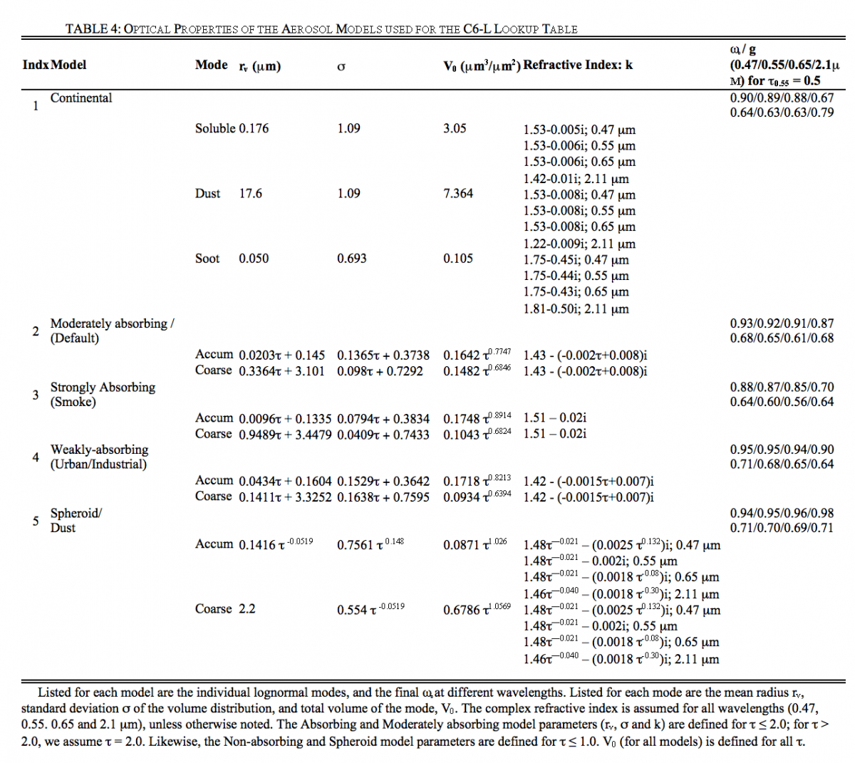
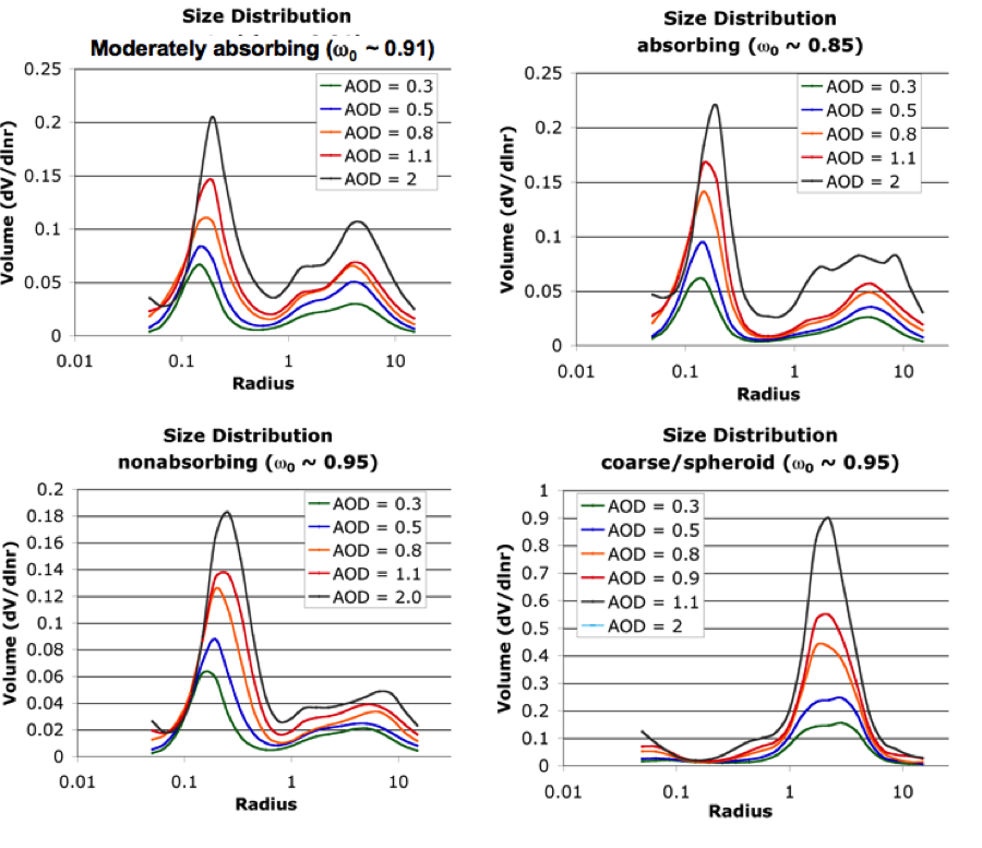
Figure 8: Aerosol size distribution as a function of optical depth for the three spherical (moderately absorbing, absorbing and non-absorbing) and spheroid (dust) models identified by clustering of AERONET.
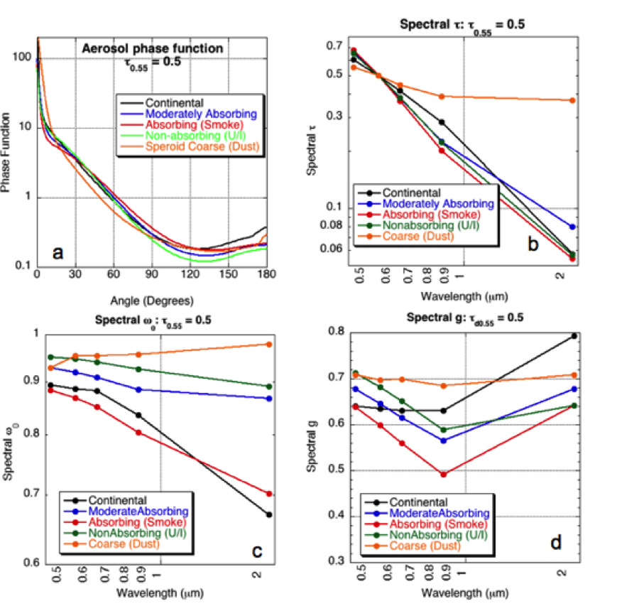
Figure 9: Plot of optical properties for the 5 aerosol models of the C5-L LUT, for τ = 0.5. a) phase function at 0.55 μm (as a function of angle) b) optical depth spectral dependence, c) single scattering albedo spectral dependence and d) asymmetry parameter spectral dependence.
The C4-L MODIS lookup table (LUT) contained simulated aerosol reflectance in two channels (0.47 and 0.65 μm), calculated using the non-polarized (scalar) SPD radiative transfer (RT) code (Dave et al., 1970). Levy et al., (2004) demonstrated that under some geometries, neglecting polarization could lead to significant errors in top of atmosphere reflectance, further leading to significant errors in τ retrieval. Figures 10a and 10b are taken from Levy et al., (2004), plotting errors in 0.47μm reflectance and associated errors in τ retrieval at the eight sun/surface/satellite geometries given in Table 5. As some errors are large (up to 0.01 for reflectance and 0.1 for τ ), it was decided to use a vector RT code for creating the C5-L LUT. Fig. 11 shows the differences between the scalar versions of Dave and RT3 (Evans and Stephens, 1991), when simulating the Continental aerosol model (see Table 5). Plotted are the differences in 0.466 μm reflectance for the eight scattering geometries of Table 5. Under most geometries and optical depths, differences between the two RT codes are less than 0.001 (which is about 1%). Note that as in Levy et al., (2004), the aerosol scattering phase function elements (inputs to RT3) were calculated by the MIEV Mie code (Wiscombe et al., 1980).
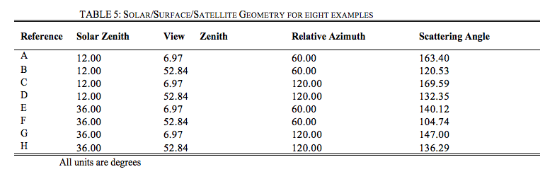
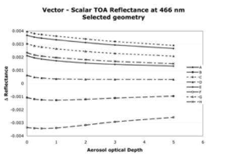
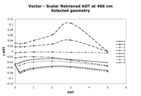
Figure 10: Difference between vector- and scalar- derived reflectance (a - top) and retrieved τ (b - bottom) at 0.466 μm, for eight example sun/surface/satellite geometries as a function of the input τ.
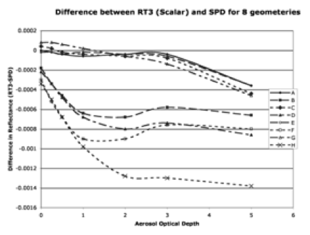
Figure 11: Difference between MIEV/RT3 combination and SPD derived reflectance at 0.466 μm, for eight example sun/surface/satellite geometries as a function of the input τ.
As described above, the fine aerosol models are assumed to be spherical particles. We used the combination of MIEV (Wiscombe et al., 1980) and RT3 (Evans and Stephens, 1991), described above and by Colarco et al., (2003). For the spheroids of the coarse aerosol model, Mie theory is not sufficient. We used instead, a version of the T-matrix code described in Dubovik et al., (2002, 2005), to calculate the scattering properties of the model. Not only is this a necessary approximation for integrating a spheroid size distribution, it is consistent with the calculations used in fitting the original almucantur radiance in the first place. In summary, then, a combination of the T-matrix and RT3 codes is used for the coarse (dust) model LUT. Assumed central wavelengths and Rayleigh optical depths are shown in Table 1. The C5-L LUT contains pre-computed optical properties of aerosol at four discrete wavelengths (0.466, 0.553, 0.644 and 2.119 μm, representing MODIS channels 3, 4, 1 and 7, respectively) for several values of aerosol total loadings, and for a variety of geometry. For discrete optical depths (described by the τ or τ at 0.55 mm) each spherical aerosol model (Continental, Moderately Absorbing, Absorbing and Non-absorbing) and non-spherical model (Dust), scattering/extinction properties of aerosol size distributions are calculated by either MIEV or the Dubovik T-matrix code. Assuming a Rayleigh atmosphere and realistic layering of the aerosol, the Legendre moments of the combined Rayleigh/aerosol are computed for each layer of a US Standard Atmosphere (U.S. Government, 1976). These moments are fed into RT3 to simulate TOA reflectance and total fluxes.
The parameters of Equation (28) were calculated for seven aerosol loadings (τ0.55 = 0.0, 0.25, 0.5, 1.0, 2.0 3.0, and 5.0). TOA reflectance was calculated for 9 solar zenith angles (θ0 = 0.0, 6.0, 12.0, 24.0, 36.0, 48.0, 54.0, 60.0 and 66.0), 16 sensor zenith angles (θ = 0.0 to 65.0, approximate increments of 6.0), and 16 relative azimuth angles (Φ= 0.0 to 180.0 increments of 12.0). All of these parameters are calculated assuming a surface reflectance of zero. The approximate increments of θ arise from the use of the Lobatto quadrature function in RT3; allowing for values that resemble C004-L LUT without having to perform extra interpolation.
When surface reflectance is present, the second term in Equation (28) is nonzero. The flux is a function only of the atmosphere, however, the atmospheric backscattering term, s, and the transmission term, T, are functions of both the atmosphere and the surface. Therefore, RT3 is run two additional times with distinct positive values of surface reflectance.
 (29 a, b)
Here, we chose values of 0.1 and 0.25 for our surface reflectance. ρ s1 and ρ s2. These two equations can be solved for the two unknowns, s and T. The values of Fd, s, and T are saved into the LUT, for each τ index, wavelength and aerosol model.
Other parameters contained in the LUT include the scattering and extinction coefficients Q and variables describing the physical properties (lognormal size parameters rg and σ, and complex refractive indices, nr+ink) of the aerosol models. We also compute a Mass concentration coefficient, MC, in units of (μg per cm2) that is a function of optical thickness and Q. The derivation of MC and some typical values are explained in Appendix 3.
5.4 VIS vs 2.11 surface reflectance assumptions
When performing atmospheric retrievals from MODIS or any other satellite, the major challenge is separating the total observed reflectance into atmospheric and surface contributions, and then defining the aerosol contribution. Over the ocean, the surface is nearly black (non-reflecting) at red wavelengths and longer, so that assuming negligible surface reflectance in these channels is a good approximation. Over land, however, the surface reflectance in the visible and SWIR is far from zero and varies over surface type. As the land surface and the atmospheric signals are comparable, errors of 0.01 in assumed surface reflectance will lead to errors on the order of 0.1 in τ retrieval. Errors in multiple wavelengths can lead to poor retrievals of spectral τ, which in turn would be useless for estimating size parameters.
Kaufman and colleagues (e.g. Kaufman et al., 1997b) observed that over vegetated and dark soiled surfaces, the surface reflectance in some visible wavelengths correlated with the surface reflectance in the SWIR. Parallel simulations by vegetation canopy models, showed that the physical reason for the correlation was the combination of absorption of visible light by chlorophyll and infrared radiation by liquid water in healthy vegetation (Kaufman et al., 2002). These relationships were such that the surface reflectance values in the visible (blue and red channels) were nearly fixed ratios of that in the SWIR (Kaufman et al., 1997c). As applied within C4-L (and all previous versions), surface reflectance in the blue (0.47µm, channel 3) and the red (0.65 µm, channel 1) channels were assumed to be one-quarter and one-half, respectively, of the surface reflectance in the mid-SWIR (2.1µm, channel 7) channel (Kaufman et al., 1997b). We note these as the ‘0.47vs2.11’ and ‘0.65vs2.11’ ratios, respectively, and collectively as ‘VISvs2.11’
However, correlation of C4-L (and prior) MODIS-derived t to AERONET sunphotometer data (Chu et al., 2002; Remer et al., 2005) showed a positive offset of about 0.1, likely meaning that the surface reflectance was under-estimated. From data observed during the CLAMS experiment of 2001, Levy et al., (2005) demonstrated that higher values of VISvs2.11 surface ratios (e.g. 0.33 and 0.65 for the blue and red, respectively) improved the continuity of the MODIS over-land and over-ocean aerosol products along the coastline of the DelMarVa Peninsula. The MODIS/AERONET τ regression over near-coastal sites was also improved. However, at locations far from the coastline, the CLAMS VISvs2.11 ratios tended toward over-correction of the surface reflectance and retrievals of τ less than zero. It is also known that earth’s surface is not Lambertian, and that some surface types exhibit strong bi-directional reflectance functions (BRDF). Gatebe et al., (2001) flew the Cloud Absorption Radiometer (CAR) low over vegetated surfaces and found that the VISvs2.11 surface ratios varied as a function of angle, and often greatly differed from the one-quarter and one-half ratios assumed in C4-L. Remer et al., (2001) also noted that the VISvs2.11 surface ratios varied as a function of scattering geometry. In fact, under certain geometry, these VISvs2.11 surface ratios broke down completely. Some of this is related to BRDF effects (e.g. Lyapustin et al., 2001).
To understand how VISvs2.11 surface reflectance relationships vary by location, season and angle, we performed atmospheric correction on the co-located C4-L-MODIS/AERONET data. Atmospheric correction (Kaufman and Sendra, 1988) attempts to calculate the optical properties of the surface, by theoretically subtracting the effects of the atmosphere from the satellite-observed radiation field. The atmospherically corrected surface reflectance ρ sλ is calculated by re-arranging Equation (28). In order to minimize errors arising from multiple scattering, we limited our exercise to conditions of τ in the green less than 0.2. Out of the original 15,000 co-located MODIS/AERONET points (described in section 2), there are over 10,000 collocations which meet this condition. The archive contains “gas absorption corrected” MODIS-Level 2 observed reflectance (see Appendix) and AERONET-observed spectral τ, column water vapor depth. For each MODIS parameter, four statistical parameters are reported, including: ‘pval’ (value for the central pixel-closest to the sunphotometer), ‘npix’ (number of valid retrievals within a 5 x 5 box; ≤ 25), ‘mean’ and ‘sdev’ (mean and standard deviation within the box). For each AERONET parameter, the analogous statistics are: ‘pval’ (value for the AERONET retrieval closest in time to MODIS overpass), ‘nval’ (number of valid retrievals within one hour of overpass; ≤ 5), ‘mean’ and ‘sdev’. For the atmospheric correction, we used the pval values of MODIS spectral reflectance, and the mean values of AERONET τ and water vapor. The molecular properties of the atmosphere are assumed those of the U.S. standard atmosphere. The sea level Rayleigh optical depth (ROD) values are assumed for each MODIS spectral channel, and scaled according to the elevation/air pressure of the sunphotometer.
The relation between the satellite-measured reflectance and the surface reflectance is a complicated function of the atmospheric effects of scattering and absorption by the aerosol. Previous atmospheric correction exercises often assumed some form of the Continental aerosol model (e.g. Vermote et al., 1997), to describe both the scattering and absorption properties. While this model may provide reasonable simulations in channels near to 0.55 μm (such as 0.47 and 0.65 μm), it cannot be expected to provide accurate simulations at 2.11 μm, even for low τ. For example, for τ0.55 = 0.2, τ2.11 ranges from 0.03 to 0.16, depending on which of our aerosol types are assumed. Thus, assuming the wrong aerosol size in the correction procedure will lead to errors in estimating 2.11 μm surface reflectance.
The LUT spectral reflectance is interpolated for geometry and AERONET measured τ, thus estimating TOA reflectance over a black surface (path reflectance). From the AERONET-derived Ångstrom exponent, we can decide whether to assume a fine model or a coarse model. Since ω 0 is not known, the moderately absorbing/developing world aerosol type (ω 0 ~ 0.9) was chosen to represent fine-dominated aerosol. When α < 0.6 (400 cases), the correction procedure assumed the coarse-dominated model. Co-locations where 0.6 < α < 1.6 (about 6000 cases) were not used due to uncertainties of aerosol mixing.
The atmospheric correction resulted in two datasets: surface reflectance at three wavelengths (0.47, 0.65, 2.11 µm) for each of the two regimes (fine and coarse-dominated). Separate comparison of 0.65 μm versus 2.11 μm and 0.47 μm versus 2.11 µm, for each regime indicated that their regressions differed by less than 10% (both slope and y-offset values), therefore the two surface reflectance datasets were combined into one.
Figure 12a plots the entire set of atmospherically corrected visible surface reflectance (in the blue ρs0.47 and the red ρs0.66) versus that in the mid-SWIR (ρs2.12) and their regression lines. While not included here, also considered were the regressions if they were forced through zero, thereby assuming that zero SWIR reflectance is zero reflectance over the entire spectrum (which would be equivalent to deriving simple ratios). Correlation (R) values are 0.93 for the red, but only about 0.75 for the blue. In the blue, forcing a regression through zero produces very different results than if the regression is not constrained. If forced through zero, the slope tends toward about 0.36, whereas including the offset (about +0.011) yields a slope closer to the assumed one-quarter (0.258). In the red, whether including offset or not, the slope is about 0.55. Thus in a mean sense, atmospheric correction of MODIS data yields VISvs2.11 surface reflectance relationships that differ from the assumed C4-L VISvs2.11 ratios. Figure 12b shows that fitting blue to red (0.47vs0.65) has higher correlation and less scatter than 0.47vs2.1 directly, suggesting a better relationship between the two visible channels. There is less difference between fitting through zero and not, such that a straight blue/red ratio is about 0.54, and the full regression has slope = 0.508 and offset = 0.008. Therefore, instead of the 0.47 μm and 0.65 μm surface reflectance being calculated separately from 2.11 μm, we calculate the 0.65 μm surface reflectance from that in 2.11 μm, followed by calculating 0.47 μm from the 0.65 μm, i.e.
 (30)
(30)
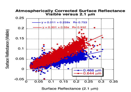
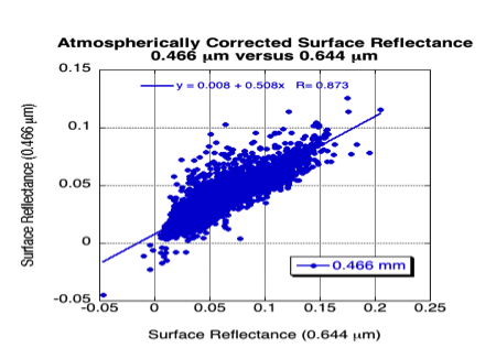
Figure 12: Atmospherically corrected surface reflectance in the visible (0.47 and 0.65 μm channels) compared with that in the 2.11 μm SWIR channel (a), and the 0.47 μm compared with that in the 0.65 μm channel (b).
As noted in Figures 12a and 12b the VISvs2.11 surface reflectance regressions display large scatter. For example, if surface reflectance is 0.15 at 2.11 μm, applying the regressed relationships of 0.65vs2.11 and 0.47vs0.65 results in estimates of surface reflectance of 0.083±0.03 at 0.65 μm and 0.050±0.03 at 0.47 μm. Obviously, this could result in very large errors in retrieved τ, on the order of 0.3 or more. Therefore, to reduce the scatter we look for dependencies on other parameters to refine the relationships.
The works of Gatebe et al. (2002) and Remer et al. (2001) suggests that the VISvs2.11 surface reflectance relationships are angle dependent. We tested which type of angle (solar zenith angle, sensor zenith angle, glint angle or scattering angle) most affected the VISvs2.11 surface reflectance relationship. The highest correlation of the VISvs2.11 surface variability was found to be with scattering angle Θ, defined as:
 (31)
(31)
where θ0, θ and Φ are the solar zenith, sensor view zenith and relative azimuth angles, respectively. Figure 12 (a) displays the median values of surface reflectance as a function of scattering angle, and shows a definite relationship at 2.11 μm, less at 0.65 μm, and nearly none at 0.47 μm. Since Figures 12a and 12b showed that both a slope and y-offset was necessary to regress VIS to 2.11 μm surface reflectance, we look for scattering angle dependence on both parameters. Fig 12 (b-d) plots the slope, y-offset and correlation of the surface reflectance relationships, as a function of scattering angle. The 0.66vs2.11 regression slope shows dependence on scattering angle, whereas the 0.47vs0.65 regression slope shows nearly none. The regressed y-intercept shows strong dependence on scattering angle for both relationships. Especially interesting is that the 0.65vs2.11 y-offset goes from positive to negative with increasing scattering angle, with a value of zero near Θ =135°.
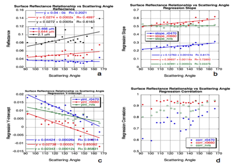
Figure 13: VISvs2.11 surface reflectance relationships as a function of scattering angle. The data were sorted according to scattering angle and put into 20 groups of equal size (about 230 points for each scattering angle bin). On all subplots, each point is plotted for the median value of scattering angle in the bin. Part (a) plots median values of reflectance at each channel as a function of the scattering angle. Linear regression was calculated for the 230 points in each group. The slope of the regression (for each angle bin) is plotted in (b), the y-intercept is plotted in (c) and the regression correlation is plotted in (d). Note for (b), (c) and (d) that 0.47 μm vs 2.11 μm (r0470) is plotted in blue, 0.65 μm vs 2.11 μm (r0660) is plotted in red and 0.47 vs 0.65 μm (rvis) is plotted in green.
Because AERONET sites are located in different surface type regimes, it could be expected that the VISvs2.11 surface relationships will vary based on surface type and/or season. Using the International Geosphere/Biosphere Programme’s (IGBP) scene map of USGS surface types and formatted for MODIS validation, we determined the scene type of the MODIS/AERONET validation box. We then separated urban from non-urban surfaces, and grouped into season (winter or summer) and general location (mid-latitude or tropical). Figures 14 and 15 display some of the surface reflectance relationships as a function of different regions and locations. Generally, “greener” surfaces (midlatitude summer sites both urban and nonurban) have higher red to SWIR ratios (red/SWIR>0.55) than winter sites (red/SWIR<0.55). Many of the AERONET sites in the tropics are in savanna or grassland regions, where the landscape is not as green, and hence the red to SWIR ratios are also lower. As for the blue to red channel surface reflectance relationships, except for the urban sites during summer (blue/red ratio ~ 0.766), the relationships around the globe are relatively consistent (blue/red ~ 0.52).
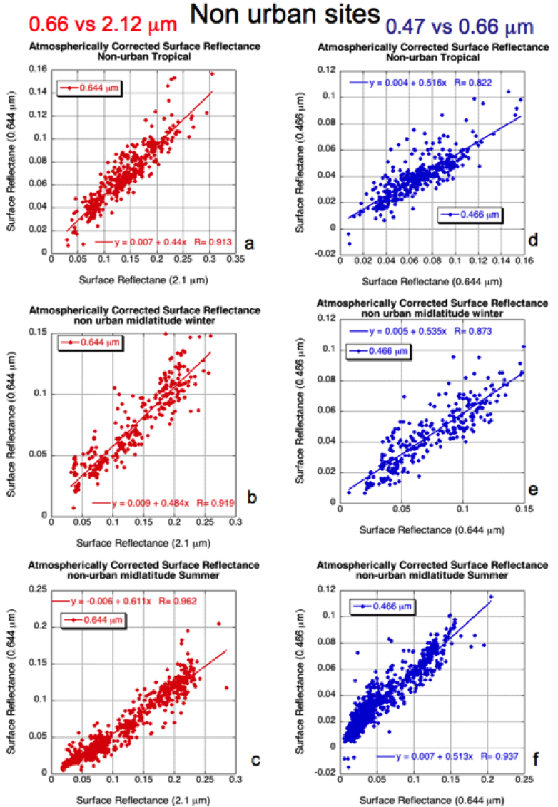
Figure 14: Surface Reflectance relationships for non-urban sites. The left three subfigures (a-c) are for Visible versus 2.11 mm channels, whereas the right three subfigures (d-f) are for 0.47 mm versus 0.65 mm channels. From the top to bottom, subfigures (a) and (d) are for tropical sites, (b) and (e) are for midlatitude sites in winter, and (c) and (f) are for midlatitude sites during summer.
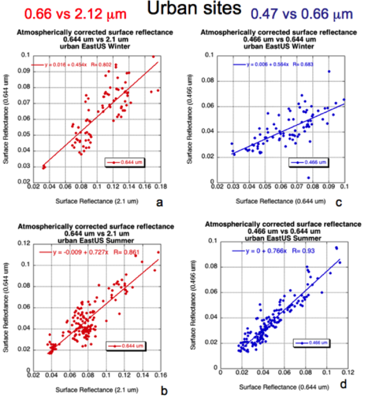
Figure 15: Surface Reflectance relationships for urban sites along the US East Coast. The left two subfigures (a-b) are for 0.65 μm versus 2.11 mm channels, whereas the right two subfigures (c-d) are for 0.47 μm versus 0.65 μm channels. From the top to bottom, subfigures (a) and (c) are for the sites in winter, and (b) and (d) are for the sites during summer.
Except for urban areas, most surfaces seem to have VISvs2.11 surface reflectance relationships that vary as a function of their “greenness.” We attempted to work with several different vegetation indices to quantify these relationships and found the most promising to be NDVISWIR, since it is not sensitive to aerosols. It is defined as:
 (32)
(32)
where ρ1.24 and ρ2.11 are the MODIS-measured reflectances of the 1.24 μm channel (MODIS channel 5) and the 2.1 μm channel (channel 7), which are much less influenced by aerosol (except for heavy aerosol or dusts). This index is also known as NDVIMIR (Mid-InfraRed). In aerosol free conditions NDVISWIR is highly correlated with regular NDVI. A value of NDVISWIR > 0.6 is active vegetation, whereas NDVISWIR < 0.2 is representative of dormant or sparse vegetation. Figure 16 plots the relationship of 0.65 μm channel and 2.11 μm channel (atmospherically corrected) surface reflectance relationship, for nonurban sites, as a function of low, medium and high values of NDVISWIR. Clearly, as the NDVISWIR increases, the ratio between 0.65 mm and 2.11 μm surface reflectance increases, and we will use this relationship in the final VISvs2.11 surface reflectance parameterization. Since the 0.47vs0.65 relationship does not strongly vary as a function of NDVISWIR, we assume it to be constant.
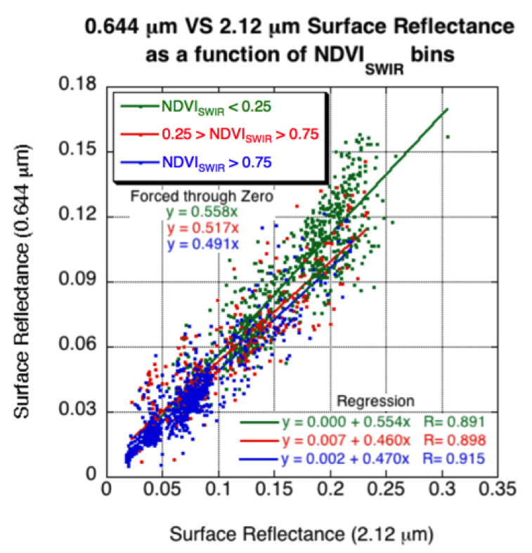
Figure 16: 0.65 μm versus 2.11 μm surface reflectance as a function of bins of NDVISWIR values (low, medium and high). Both standard regression and “forced through zero” are plotted.
Results of the global atmospheric correction exercise imply that not only do the VISvs2.11 surface relationships differ from the C4-L VISvs2.11 ratios, they also have a strong dependence on both geometry and surface type. The C5-L VISvs2.11 surface reflectance relationship is parameterized as a function of both NDVISWIR and scattering angle Θ, such that Equation (29) can be expanded:
 (33)
(33)
where
 (34)
(34)
where in turn
 (35)
(35)
Note that while the above parameterization was based on the results of Figures 11, 12 and 15, the coefficients are not identical to those in the figures. The atmospherically corrected data set is the broadest and most comprehensive representation of global surface reflectance relationships available to us. However it is limited to AERONET site locations, which are in turn are most concentrated in certain geographical regions. Trial and error was used to modify the basic results from the AERONET-based atmospheric correction, to give more realistic MODIS retrievals globally, especially in areas wtih few or no AERONET sites.
The C5 MODIS land product did not compare as well to AERONET in regions with brighter surfaces and/or mountainous terrain (e.g., US southwest, Mongolia, etc.). As the algorithm is tuned towards dark, vegetated targets, this result was not surprising. However, given that the MODIS data set had doubled since 2005 and AERONET included many new sites, we attempted to reformulate the assumed surface spectral VISto2.1 relationship (Kaufman et al., 2005; Levy et al., 2007b). Similar to the procedure described above, atmospheric correction was performed over the entire collection of MODIS/AERONET collocations. There were differences between these results and those using the 2005 database. However, any attempt to tune a new parameterization relating VIS surface reflectance to 2.11 μm reflectance using these new results introduced no improvement compared to C5.
However, even though theoretically the land surface parameterization will remain unchanged from C5-L, in practice, a large change is implemented in C6-L. On more than one occasion, the MODIS data users have inquired about the validity of the NDVISWIR in estimating the VISto2.1 relationships. Personal communications (L. Yang, 2012; P. Gupta, 2011) had suggested that Equation 32 was not coded correctly into the C5 software; this was confirmed has been fixed for C6. The bug affected how the assumed surface reflectance is dependent on NDVISWIR. Fixing the bug creates a large change in the retrieved AOD and introduces a distinctive spatial pattern in which AOD increases over vegetated surfaces and decreases over arid surfaces.
5.5 Retrieval Algorithm
A major limitation of C4-L was that aerosol is assumed to be transparent in the 2.11 μm SWIR channel. Consequently the surface reflectance in 2.1 μm was assumed to be exactly the value of the observed TOA reflectance in that channel. Under a dust aerosol regime, aerosol transparency is an extremely poor assumption. Even in a fine aerosol dominated regime, τ is not zero at 2.11 μm . For example, in our ‘moderately absorbing/developing world’ (ω0 ~ 0.9) aerosol, τ0.55 of 1.0 corresponds to τ2.11 of 0.114. For a given angle (say θ0 = 36°, θ= 36°, and Φ = 72°) assuming τ2.11 = 0.0 instead leads to error in 2.11 μm path reflectance of about 0.012. Via the VISvs2.11 reflectance relationship, the reflectance error at 0.65 μm would be on the order of 0.006, leading to ~ 0.06 error in retrieved τ. As a percentage of the actual τ, the error is not very large. However, combined with errors at 0.47 μm, the resulting incorrect Ångstrom exponent leads to error in estimating η.
Following the framework of the MODIS aerosol over ocean algorithm (Tanré et al., 1997; Levy et al., 2003; Remer et al., 2005), we developed a multi-channel reflectance inversion for retrieving aerosol properties over land, known as the “second-generation algorithm” (Levy et al., 2007b). Analogous to the ocean algorithm’s combination of fine and coarse aerosol modes, the land algorithm attempts to combine fine-dominated and coarse-dominated aerosol models (each composed of multiple modes) to match with the observed spectral reflectance. The 2.1 μm channel is assumed to contain both surface and aerosol information, and the visible surface reflectance is a function of the parameterized VISvs2.11 surface reflectance relationships. Simultaneously inverting the aerosol and surface information in the three channels (0.47 μm, 0.65 μm and 2.11 μm) yields three parameters: τ (τ0.55), the η (η0.55 ) and the surface reflectance (ρs2.11).
We rewrite Equation 28, but note that the calculated spectral total reflectance ρ*λ at the top of the atmosphere is the weighted sum (η) of the spectral reflectance from a combination of fine and coarse –dominated aerosol models, i.e.
 (36)
(36)
where r*fλ and r*cλare each composites of surface reflectance rsλ and atmospheric path reflectance of the separate aerosol models. That is:
 (37)
(37)
where ρ af λ and ρ ac λ are the fine and coarse model atmospheric path reflectance, Ffd λ and Fcd λ are normalized downward fluxes for zero surface reflectance, τf λ and τcλ represent upward total transmission into the satellite field of view, and sf λ and scλare atmospheric backscattering ratios. Note the angular and τ dependence of some of the terms: ρ a= ρ a(τ, θ 0, θ,Φ), F=F(τ ,θ0), T=T(τ ,θ), s = s(τ ) and ρ s= ρ s(θ0, θ, Φ). Whereas the other terms are a function of the aerosol and are contained within the lookup tables, the surface reflectance is independent. However, we know the VISvs2.11 surface reflectance relationships.
Due to the limited set of aerosol optical properties in the lookup table, the equations may not have exact solutions, and solutions may not be unique. Therefore, we find the aerosol solution most closely resembling the set of MODIS measured reflectances. In order to reduce the possibility of non-unique retrievals we only allow discrete values of η. During the retrieval, the algorithm tests whether certain criteria are met for consistency and valid retrieval steps. Results of these tests are encoded into a product called the ‘Quality_Assurance_Land’. Upon completion, the retrieval is assigned a final Quality Assurance confidence (QAC) value that ranges from 0 (bad quality) to 3 (good quality). Details of the QA and QAC are given in the Appendix. In the following subsections, we describe the mechanics of the inversion algorithm in more detail.
Selection of "dark pixels"
Figure 17 illustrates the main steps of the C6-L land algorithm. The relevant Level 1 B (L1B) data include calibrated spectral reflectance in eight wavelength bands at a variety of spatial resolutions, as well as the associated geo-location information. The spectral data include the 0.65 and 0.86 mm channels (MODIS channels 1 and 2 at 250 m resolution), the 0.47, 0.55, 1.2, 1.6 and 2.1 mm channels (channels 3, 4, 5, 6 and 7 at 500 m), and the 1.38 μm channel (channel 26 at 1 km). The geo-location data are at 1 km and include angles (θ, Φ, and Θ), latitude, longitude, elevation and date. The L1B reflectance values are corrected for water vapor, ozone, and carbon dioxide (described in Appendix I) before proceeding.
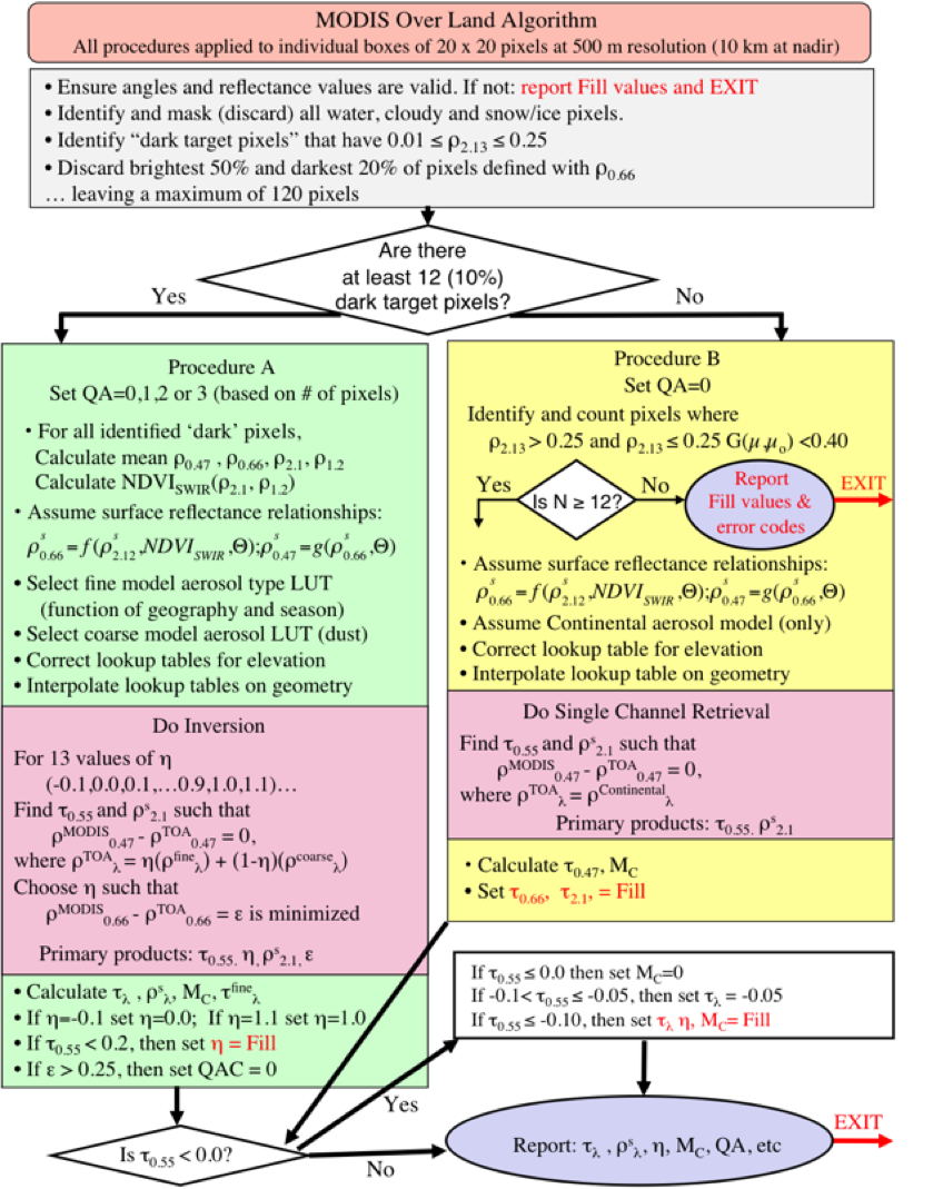
Figure 17: Flowchart illustrating the derivation of aerosol over land for C6-L.
The first step is to organize the measured reflectance into nominal (at nadir) 10 km by 10 km boxes (corresponding to 20 by 20, or 40 by 40 pixels, depending on the channel). The 400 pixels in the box are evaluated pixel by pixel to identify whether the pixel is suitable for aerosol retrieval. Clouds (Martins et al., 2002), snow/ice (Li et al., 2004) and inland water bodies (via NDVI tests) are considered not suitable and are discarded (masked). Details of masking are also described in Appendix 2. Note that while the number of pixels ramains constant across the measurement swath, the size of the pixels and therefore the retrieval boxes, increase as they approach the swath edge.
The non-masked pixels are checked for their brightness. Pixels having 2.11 μm measured reflectance between 0.01 and 0.25 are grouped and sorted by brightness. The brightest 50% and darkest 20% are discarded, in order to reduce cloud and surface contamination and scale towards darker targets. Assuming no pixels are masked in the initial screening this leaves a theoretical maximum of 120 pixels on which to perform the retreival. If there are at least 12 pixels remaining (10% of 30% of the original 400), then the reflectance in each channel is averaged, yielding the ‘MODIS-measured’ spectral reflectance ρm0.47, ρm0.65, ρm2.11, and ρm1.24. These reflectance values are used for ‘Procedure A’. If less then 12 pixels remain, then ‘Procedure B’ (described later) is followed and QAC is lowered to zero.
Correcting the LUT for elevation
The sea-level Rayleigh optical depth (ROD, tR,λ) at a wavelength λ (in mm) can be approximated over the visible range (e.g. Dutton et al., 1994; Bodhaine et al., 1998) by:
 (38)
(38)
When not at sea level (pressure = 1013 mb), the ROD is a function of pressure (or height, z) so that it can be approximated by:
 (39)
(39)
where Z is the height (in kilometers) of the surface target and 8.5 km is the exponential ‘scale height’ of the atmosphere. The difference between ROD at z=0 and z=Z is ΔτR λ .
In C4-L, the algorithm (too) simply corrected the retrieved t product by adding the optical depth that was neglected by assuming sea level for the retrieval, (i.e. τλ(z=Z) = τ λ(z=0)+ ΔτR λ). However, this correction can give poor results because of the large differences between molecular and aerosol phase functions.
Instead, the C5-L/C6-L algorithm makes use of the procedure described in Fraser et al., (1989). The algorithm adjusts the lookup table to simulate different ROD by adjusting the wavelength. Substitution of Equation (38) into equation (39) yields
 (40)
(40)
For example, at Z = 0.4 km, l increases by about 1.2%. For the blue 0.47 μm channel, (centered at 0.466 μm) this means that τR λ(z=0)=0.1918, τR λ(z=0.4)=0.185 and λ(z=0.4)=0.417μm. In other words, the algorithm simulates an elevated surface by adjusting the blue channel’s wavelength to 0.471 μm. Assuming that gases and aerosols are optically well mixed in altitude, the algorithm substitutes for the parameter values of the 0.47 μm LUT by interpolating (linearly as functions of log wavelength and log parameter) between the 0.47 μm (0.466 mm) and the 0.55 μm (0.553 μm) entries. Similar interpolations are performed for the other channels (for example, 0.55 μm would be adjusted to 0.559 μm). For the 0.4 km case, this means that lower values of TOA atmospheric path reflectance and higher values of transmission are chosen to represent a given aerosol model’s optical contribution. However, also note that since the 0.55 μm channel has also been adjusted, the associated values of the t indices have been adjusted accordingly.
Whereas most global land surfaces are at sea level or above, a few locations are below sea level (Z < 0). In these cases, the algorithm is allowed to extrapolate below 0.466 μm. Since the extrapolation is at most for a hundred meters or so, this is not expected to introduce large errors, and these cases can still be retrieved. Due to the extremely low ROD in the 2.11 μm channel we do not adjust this value.
Procedure A: Inversion for dark surfaces
If following Procedure A (for dark surfaces), the QA confidence (QAC) is initially set to a value between 0 (‘bad quality’) and 3 (‘good quality’), depending on the number of dark pixels remaining. In Procedure A, the algorithm assigns the fine aerosol model, based on the location and season (Figure 10). From the lookup table, ρa, F, T and s (for the fine model and coarse model separately) are interpolated for angle, resulting in six values for each parameter, corresponding to aerosol loading (indexed by τ at 0.55 μm).
The 2.11 mm path reflectance is a non-negligible function of the τ, so that the surface reflectance is therefore also a function of the τ. For discrete values of η between -0.1 and 1.1 (intervals of 0.1), the algorithm attempts to find the τ at 0.55 μm and the surface reflectance at 2.11 μm that exactly matches the MODIS measured reflectance at 0.47 μm. (Note that non-physical values of h are tried (1.1 and -0.1) to allow for the possibility of inappropriate assumptions in either aerosol models or surface reflectance.) There will be some error, ε, at 0.65 μm. The solution is the one where the error at 0.65 μm is minimized. In other words,

 (41 a, b, c)

where
 (42 a, b, c)
where in turn, ρa=ρa(t), F=F(τ), T=T(τ), s = s(τ) are functions of t indices in the lookup table, and f (ρs2.11), g (ρs0.65) are described by Equations (33-35). Again, the primary products are τ (τ0.55), η (η0.55 ), and the surface reflectance (ρs2.12). The error ε is also noted.
Procedure B: Alternate retrieval for brighter surfaces
The derivation of aerosol properties is possible when the 2.11 μm reflectance is brighter than 0.25, but is expected to be less accurate (Remer et al., 2005), due to increasing errors in the VISvs2.11 relationship. However, if Procedure A is not possible, and if there are at least 12 cloud-screened, non-water pixels, satisfying
 (43)
(43)
where
 (44)
(44)
then Procedure B is attempted. In this case, QAC is automatically set to 0 (‘bad quality’).
Procedure B is analogous to ‘Path B’ described in Remer et al., (2005). As in C4-L, the Continental aerosol model is assumed. Unlike C4-L, the VISvs2.11 surface reflectance assumptions are those described by Equations (13-15) and the Continental aerosol properties are indexed to 0.55 μm. In other words, it uses equations (16-17), except with the first term only (i.e. η = 1.0). The primary products for Procedure B are τ (τ0.55) and the surface reflectance (ρs2.12). The ‘land fitting error’ ε is also saved.
Derivation of Fine Mode τ, Mass Concentration and other secondary parameters
Following the derivation of primary products by Procedure A (τ0.55, η0.55 and ρs2.12), a number of secondary products can also be calculated. These include the fine and coarse model optical depths τf0.55 and τc0.55:
 (45)
(45)
the "mass concentration", M:
 (46)
(46)
the spectral total, fine and coarse model optical thicknesses τλ, τfλ, and τcλ:
 (47)
(47)
the Ångstrom Exponent α:
 (48)
(48)
and the spectral surface reflectance ρsλ,, computed by re-arranging Equations (33-35). Mfc and Mcc are mass concentration coefficients for the fine and coarse models, whereas Qfλ and Qcλ represent model extinction coefficients at wavelength, λ. See Appendix 3 for derivation of the extinction coefficients. If the products are inconsistent, then the QAC value initially assigned to the pixel is changed to 0 (‘bad quality’), and only a subset of the products is reported.
If Procedure B was followed, the only secondary products calculated are M and τ0.47, and the QAC is set to 0. The other products are undefined.
Negative (and very low) optical depth retrievals
A major philosophical change from C4-L to C5-L was that negative τ retrievals were allowed. Given that there is both positive and negative noise in the MODIS observations, and that surface reflectance and aerosol properties may be under or over-estimated depending on the retrieval conditions, it is statistically useful to allow retrieval of negative τ. In fact it is necessary for creating an unbiased dataset from any instrument. Without negative retrievals the τ dataset is biased by definition. Negative AOD retrievals continue to be permitted in C6-L.
The difficulty here is to distinguish between a retrieved τ that is truly close to zero and an erroneous retrieved τ . Since we assume that MODIS should retrieve between the expected error defined by Equation 23 (±0.05±0.15τ) for very clean conditions when τ~0 there is essentially no difference between retrievals in the range of -0.05 to +0.05. All negative values -0.05 to 0 are reported with QAC rated ‘good’ (QAC=3). Retrievals in the range -0.10 to -0.05 are reported as -0.05. Retrievals less than -0.10 are regarded as ‘out of range’ and are not reported. Other products that are retrieved or derived (such as the η) are set to zero or reported as not defined when the retrieved τ is negative.
In cases where low τ is retrieved (τ < 0.2), the η is too unstable to be retrieved with any accuracy. Therefore, η is reported as un-defined.
5.6 Sensitivity Study
Following the lead of Tanré et al (1997), we have tested the sensitivity of Procedure A by applying it in the following exercises: (1) simulation of conditions that are included within the LUT, (2) simulations where one of the parameters (i.e. τ) is not included within the LUT, and (3) simulations for conditions that include one or more errors.
Whereas the study of Tanré et al, (1997) tested the algorithm on a single geometrical combination, we performed the study in (1) by simulating the 720 reasonable geometrical combinations in the LUT (0°≤Φ≤180°, θ≤60°, θ0≤48°). We assumed the “fine” aerosol model to be the moderately absorbing (ω0~0.9) aerosol model and that the “coarse” model was our Spheroid (dust) model. For each combination of geometry, and for each MODIS channel, we extracted the fine and coarse mode values of atmospheric path reflectance ρal, backscattering ratio sλ, downward flux Fd and transmission Tλ. We assumed a 2.1 μm surface reflectance of ρs2.12 = 0.15, and the C4-L VISvs2.11 surface reflectance ratios (i.e, ρs0.66= 0.5 ρs2.12 and ρs0.47= 0.5ρs0.66). Using Equations (16-17), we simulated TOA reflectance ρ*λ for 5 discrete values of the η (η = 0.0, 0.25, 0.5, 0.75 and 1.0). Therefore, for each value of τ in the LUT, there are 720 x 5 = 3600 attempts to retrieve that τ.
Figure 18 plots the mean (open circles) and standard deviation (error bars) of retrieved τ, as a function of the input τ. For smaller τ (τ ≤ 1), the τ was retrieved nearly perfectly. As τ increases computational instabilities lead to a less exact solution however the retrieved τ is still within 10%. It is interesting to note that the algorithm tends to over-estimate τ for these higher values.
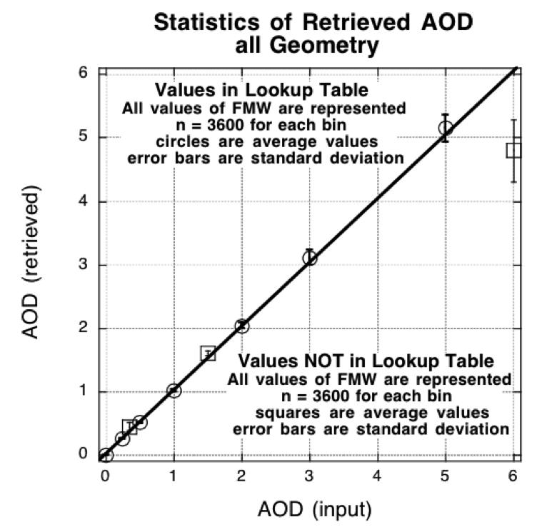
Figure 18: Scatter diagram of the retrieved τ (AOD) versus the input τ. The open shapes correspond to the average of the solutions for each inputted τ, where there are 3600 combinations of geometry and input η (FMW in the figure). The error bars are the standard deviation of the 3600 inputs. The open circles represent cases where the inputted τ are included in the C5-L lookup table, whereas the open squares represent inputted τ that are not in the LUT.
Figure 19 shows attempted retrievals of η when the τ is held constant at τ = 0.5 (for all 720 geometrical combinations). η of 0.0 and 1.0 can be considered to be exactly within the LUT, and are retrieved nearly perfectly. The algorithm is limited to determining η in 0.10 increments.
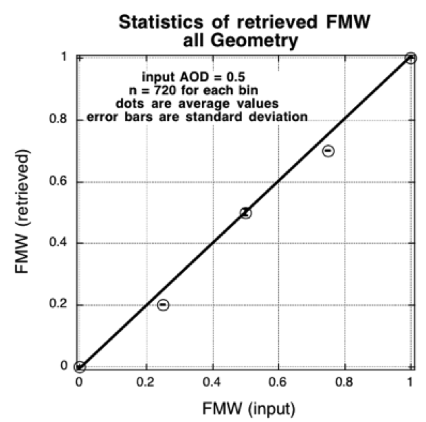
Figure 19: Scatter diagram of the retrieved η (FMW) versus the input η. The open shapes correspond to the average of the solutions for each inputted η, where there are 720 combinations of geometry and input τ (AOD). The error bars are the standard deviation of the 720 inputs. Only the η values of 0.0 and 1.0 would be represented exactly in the LUT, as all coarse and all fine model, respectively. Note the cases for which input η=0.25 and η=0.75, where the algorithm is only allowed to determine η in 0.10 increments.
Figures 20 and 21 provide another way of assessing the retrieved MODIS products. Fig 20 plots retrieved τ, surface reflectance and fitting error as a function of either air mass (top) and scattering angle (bottom), given that the input conditions are τ0.55=0.5, η=0.5 and ρs2.12=0.15. In this case, we plotted all of the 720 geometrical combinations in the LUT. Note that retrieval never exactly matches the input reflectances, although the errors are very small (less than 0.1%). Also noteworthy is that the retrieval selects an under-estimated surface reflectance to balance the over-estimated optical depth. Fortunately, though, most errors are small, and are well within any expected error bars. Figure 21 is similar, but for η=0.25, and plotted only for the air mass dependence.
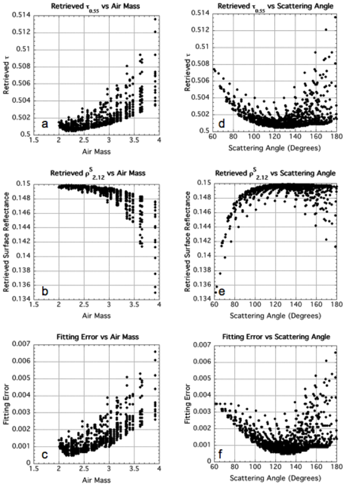
Figure 20: Retrieved MODIS products as a function of Air Mass (a-c) and Scattering Angle (d-f) for given atmospheric conditions (τ=0.5, h=0.5 and rs2.11=0.15) and 720 LUT geometrical combinations. The retrieved τ is plotted in (a) and (d), the 2.11 surface reflectance in (b) and (e) and the fitting error is plotted in (c) and (f). Note that in all cases, the η value of 0.5 was retrieved exactly.
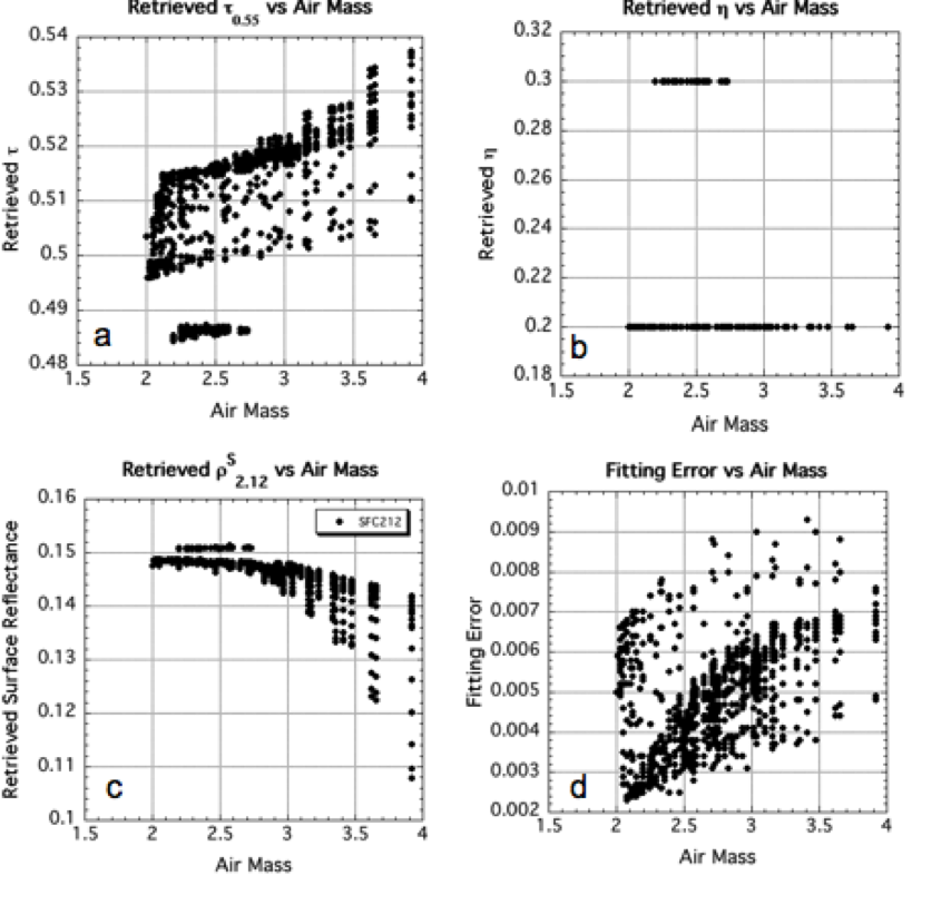
Figure 21: Retrieved MODIS products as a function of Air Mass for given atmospheric conditions (τ=0.5, η=0.25 and rs2.11=0.15) and 720 LUT geometrical combinations. The retrieved τ is plotted in (a), η in (b) the 2.11 mm surface reflectance in (c) and the fitting error is plotted in (d). Errors are much larger (up to 1%), but τ is still well within expected error.
(2) We used the same combination of radiative transfer codes (MIEV + RT3) used for the LUT to simulate additional values of aerosol loading (τ0.55 = 0.35, 1.5 and 6.0) to create an “extended” LUT. As in exercise (1) we simulated the same 720 geometrical combinations as in the C5-L LUT and the five values of η.
Also plotted in Fig 18 are the average values (open squares) and standard deviation (error bars) of the retrieved τ for conditions of this extended LUT. On average the retrieval is very close to the expected value, however, the standard deviation over all geometry is larger than for t in the normal LUT. A notable exception is the attempt at retrieving τ0.55 = 6.0, where the algorithm does a poor job of extrapolating. In the operational algorithm, we constrain the maximum possible τ to be 5.0. As for retrieving η values not included in the LUT, Figure 19 demonstrates that the algorithm is successful. The η=0.5 retrieval is well behaved. The attempt at resolving either η=0.25 or η=0.75 leads to retrieving η =0.20 and η =0.70. Although it is impossible for an exact retrieval, due to the algorithm choosing between 0.1 intervals, it is interesting that no retrievals of η=0.30 or η = 0.80 are produced.
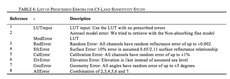
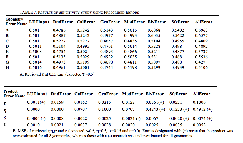
(3) This exercise studied the impact of different types of errors that could creep into the retrieval process. Potential errors include (but are not limited to) random, systematic or spectrally dependent errors that arise from issues like sensor calibration, assuming the wrong aerosol model at a given location, coarse input topography mapping, or wrong estimates of the VISvs2.11 surface reflectance relationships.These errors are expressed by adding random or systematic errors in the measurements of one or more spectral channels, geometrical conditions or other input boundary conditions. Table 6 lists some prescribed errors, whereas Table 7 shows results when attempting to retrieve conditions of τ0.55=0.5, η =0.5 and ρs2.12=0.15, for the eight sample geometries described in Table 5. Under most conditions, introducing minor calibration or random errors does not kill the retrieval. Even when introducing geo-location errors (angle or assumed aerosol model), the retrieved τ is within expected error bars. As expected, introducing multiple errors to the retrieval leads to poorer retrievals. However, the combination of all sensitivity tests shows that the C5-L algorithm is generally stable.
5.7 Retrieved land products
Examples of the three primary aerosol products (τ0.55, η and ρs2.12) are shown in Fig. 22B-D, along with a color composite (RGB image) of the L1B reflectances (0.47, 0.55 and 0.65 μm channels) in Figure 22A. This Terra image was taken over the Eastern U.S. on May 4, 2001. It shows a plume of aerosol, seemingly transported from the Ohio Valley, through Maryland, and into the Atlantic. Aerosol optical depths in the plume are high, τ0.55 ~ 1.0. The aerosol is also dominated by fine particles as seen in the η image (plotted where τ0.55 > 0.2). The land/ocean continuity is very good, and the t continuity is discussed later. AERONET observations in Baltimore (MD_Science_Center) show τ ~ 1.0 and Ångstrom exponent ~ 2.0, also indicating fine-dominated heavy aerosol.
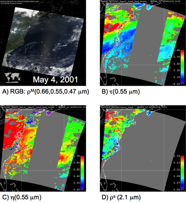
Figure 22: Retrieved aerosol and surface properties over the Eastern U.S. on May 4, 2001. This figure can be compared with that plotted in King et al., (2003). Panel A) is a ‘true-color’ composite image of three visible channels, showing haze over the mid-Atlantic. Panels B) and C) show retrieved τ and η, showing that the heavy aerosol (τ ~ 1.0) is dominated by fine particles. The transport of the aerosol into the Atlantic is well represented with good agreement between land and ocean. In fact the continuity of τ seems to be improved since earlier versions of the aerosol algorithm. Note that over-land η is not reported when τ < 0.2. Panel D) shows the retrieved surface reflectance during the retrieval.
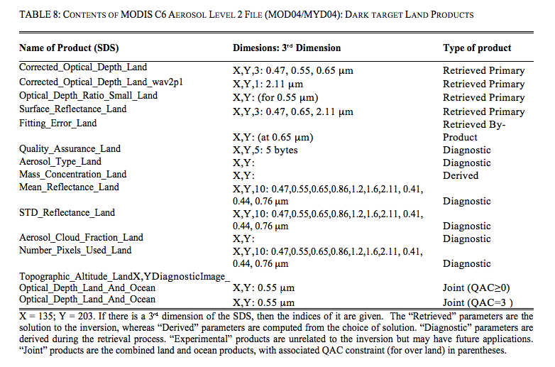
Table 8 lists the aerosol over land products that are within each “MxD04” Level 2 granule. For each product, the table lists its name within the file, its dimension, and its “type.” All products are at least two-dimensional (nominally 135 x 204 at 10 km x 10 km resolution), and many have three dimensions. If there is a third dimension, the channels (usually wavelengths) are listed. A parameter’s type may be Retrieved, Derived, Diagnostic, Experimental, or Joint Land and Ocean. A Retrieved parameter is one that is a solution to the inversion (Procedure A). Derived parameters are computed based on products directly retrieved. Products that are Diagnostic include QA parameters and those parameters that were calculated during intermediate steps.
These diagnostic parameters can be used to understand how the retrieval worked. Note that a parameter’s type does not signify that the parameter should be used in a quantitative way. Each parameter should be independently validated through comparison with ground-truth. Some provisional validation is described in section 6, however more rigorous evaluation of each parameter are subjects of future studies.
Finally, the Joint products are those that are composites of over-land and over-ocean aerosol retrievals. For example, Image_Optical_Depth_Land_And_Ocean includes all 0.55 μm τ data from ‘Corrected_Optical_Depth_Land’ including those with QAC=0. This product provides a full picture of the aerosol distribution, even if some of the retrievals are more qualitative in nature than the validated quality assured data. The ‘Optical_Depth_Land_And_Ocean’ product is designed to include the more quantitative data, and is filtered for higher QAC. Based on evaluation of the operational C5-L data stream, the recommended QAC filter used for the ‘Optical_Depth_Land_And_Ocean’ product is QAC > 0 over ocean and QAC = 3 over land.